19 Curvature
We’ve seen that in some ways the sphere behaves similarly to the plane, and in other ways its quite different. Qualitatively, the big difference stems from the lack of any similarities other than isometries: this makes there be no universal constant like \(\pi\) or \(\tau\), for one. Our goal in this chapter is to quantify that difference.
In doing so, we will uncover the precise quantity of curvature: which measures how much geometry differs from that of the flat plane. This chapter will be short, but is discovery crucially important to all geometry beyond that of Euclidean space!
19.1 Circumference of Circles
Our first real quantitative difference between the sphere and the plane had to do with the the size of circles, so this is where we begin. We know (Definition 16.1) that for circles in Euclidean space \(C=2\pi r\), and by (?exr-sphere-circle-circumference) that the analog in the sphere is \(C=2\pi\sin(r)\). Circles on the sphere grow slower than circles in the plane, as we can see by graphing these two functions.

19.1.1 Limits
But how can we turn this slower insight into something quantitative, and infinitesimal? We want to be able to measure the curvature of the sphere at a point \(p\), so we should naturally be looking not at circles of some fixed finite radius, but rather families of circles that are shrinking down centered at the point \(p\). How do these behave? Zooming in on the graph above we reach a first disappointment: it’s hard to tell their behavior apart from Euclidean circles!
This is because the series expansion of \(\sin(r)\) starts out with \(r-\frac{1}{3!}r^3+\cdots\) and so \(2\pi\sin(r)\) starts out with \(2\pi r-\cdots\) - the same as in the Euclidean case! We already knew this - that at small scales the geometry of the sphere looks Euclidean, so what we are more interested in is the difference between the two geometries: that is, we care about
\[\lim_{r\to 0}C_{\EE^2}(r)-C_{\SS^2}(r)\]
Or, at least - something like this! This can’t be the right quantity all alone as when \(r\) shrinks, both of these go to zero, and so the limit just gives zero! This problem is reminiscent of when we define the derivative in Calculus I: if we just look at the difference in \(y\) values
\[\lim_{h\to 0}(f(x+h)-f(x))\] the result goes to zero - which is not helpful! This is because we really need to be measuring a ratio - how much is this difference changing as \(x\) changes (or, in our case, as \(r\) changes).
This might suggest we take a look at the quantity
\[\frac{C_{\EE^2}(r)-C_{\SS^2}(r)}{r}\]
But if we graph this quantity as \(r\to 0\) we see this still goes to zero! In fact, the same happens if we normalize by a denominator of \(r^2\): neither of these lets us see the difference between the sphere and the plane show up in the limit yet.
However, when we normalize by \(r^3\), we actually get something that converges to a finite nonzero number!
Exercise 19.1 Check this, that as \(r\to 0^+\) the following limits both exist, and are both equal to zero: \[\lim_{r\to 0}\frac{C_{\EE^2}(r)-C_{\SS^2}(r)}{r}=0\] \[\lim_{r\to 0}\frac{C_{\EE^2}(r)-C_{\SS^2}(r)}{r^2}=0\]
But
\[\lim_{r\to 0}\frac{C_{\EE^2}(r)-C_{\SS^2}(r)}{r^3}\neq 0\] what is its value?
Hint: recall that \(C_{\EE^2}(r)=2\pi r\) and \(C_{\SS^2}(r)=2\pi\sin(r)\), and L’Hospital’s rule.
This is a number that an inhabitant of the sphere could calculate for themselves: for smaller and smaller values of \(r\) they could compute this ratio by measuring things on the sphere, and look at what value the limit is approaching. And, the fact that they do not get zero would tell them definitively that they live somewhere other than the plane!
At this point, we could just define this ratio to be the curvature, but its convenient instead to normalize it: we multiply by a normalizing constant so that the curvature of the unit sphere is equal to \(+1\):
Definition 19.1 (Curvature) If \(X\) is any surface and \(C_X(r)\) is the function which gives the circumference of the circle of radius \(r\) centered at \(p\), then the curvature at \(p\) is defined by the limit
\[\kappa(p)=\left(\frac{3}{\pi}\right)\lim_{r\to 0}\frac{C_{\EE^2}(r)-C_{X}(r)}{r^3}\]
A nice feature of this definition is that, being based totally off of lengths, its easy to check that curvature is not changed by isometries.

Theorem 19.1 If \(\phi\) is an isometry that takes \(p\) to \(q\), then \(\kappa(p)=\kappa(q)\).
Proof. Let \(\phi\) be an isometry taking \(p\) to \(q\). Then as \(\phi\) does not change distances, it takes circles of radius \(r\) (a distance) based at \(p\) to circles of radius \(r\) based at \(q\). And, as \(\phi\) doesn’t change the length of curves, it does not change the circumference of these circles.
Since the numerator and denominator of the limit expression are built purely using the distance \(r\) and circumference (and the Euclidean circumference, which is just \(2\pi r\) - a multiple of \(r\).) none of these quantities are changed by isometries, so the limit that we need to evaluate at \(p\) is the exact same limit as the one we need to evaluate at \(q\): thus we get the same number both times.
PICTURE
This has a nice corollary for homogeneous spaces: if there’s an isometry that takes any point to any other, then the curvature at every point must be the same!
Corollary 19.1 The unit sphere has constant curvature \(+1\), and the Euclidean plane has curvature \(0\).
19.1.2 Series & Derivatives
We can also approach this more algebraically than geometrically, after realizing that the correct geometric notion (a normalized difference) looks somewhat like a derivative. In particular, the series expansion of \(\sin(r)\) is \[\sin(r)=r-\frac{1}{3!}r^3+\frac{1}{5!}r^5-\cdots\]
so the series expansion of the circumference of a circle on \(\SS^2\) is
\[C_{\SS^2}(r)=2\pi r -\frac{\pi}{3}r^3+\frac{\pi}{60}r^5-\cdots\]
And so, we can see that the third series coefficient is exactly what our limit was computing! But what is the third coefficient is a series expansion? Remember Taylor’s formula:
\[f(x)=f(0)+f^\prime(0)x+\frac{f^{\prime\prime}(0)}{2!}x^2+\frac{f^{\prime\prime\prime}(0)}{3!}x^3+\cdots\]
The third coefficient is just the third derivative divided by \(3!\). So, this means we can replace our limiting expression with \(C^{\prime\prime\prime}(0)/3!\), and get a new expression for curvature:
Definition 19.2 Let \(C(r)\) be the circumference function for circles of radius \(r\) centered at a point \(p\), on some surface. Then the curvature at \(p\) is given by \[\kappa(p)=-\frac{C^{\prime\prime\prime}(0)}{2\pi}\]
Proof. This is just a computation, plugging in our new term in place of the limit:
\[\begin{align*} \kappa(p)&=\left(\frac{-3}{\pi}\right)\lim_{r\to 0}\frac{C_X(r)-C_{\EE^2}(r)}{r^3}\\ &=\left(\frac{-3}{\pi}\right)\frac{C^{\prime\prime\prime}(0)}{3!}\\ &=\frac{-1}{\pi}\frac{C^{\prime\prime\prime}(0)}{2}\\ &=\frac{-C^{\prime\prime\prime}(0)}{2\pi} \end{align*}\]
19.2 Area of Circles
We could also choose quantify the curvature of a space by comparing the area of circles to their Euclidean counterparts. Just like above, we could imagine two separate ways of extracting a quantitative number:
- A normalized limit of the difference between Spherical and Euclidean areas
- A normalized derivative of the Area Function
In both cases, we want to fix the normalizing factors so that the limit exists and the curvature comes out to be \(+1\).
Exercise 19.2 (Curvature and Area: I) Give a limit definition of the form \[\kappa =\lim_{r\to 0}\frac{\mathrm{area}_{\SS^2}(r)-\mathrm{area}_{\EE^2}(r)}{\textrm{normalizing factor}}\] which computes the curvature of the sphere. What’s the normalizing factor?
Exercise 19.3 (Curvature and Area: II) Give a limit definition of the form \[\kappa =C\cdot \frac{d^n}{dr^n}\mathrm{area}_{\SS^2}(r)\Bigg|_{r=0}\] which computes the curvature of the unit sphere. What is \(n\), what is \(C\)?
19.3 Distance Between Geodesics
Besides circles, there’s another interesting difference between the sphere and the plane we could try to quantify to measure curvature: how quickly geodesics spread out.
You are not responsible for this material now, but we will come back to it as an example when discussing the differences between spherical and hyperbolic space

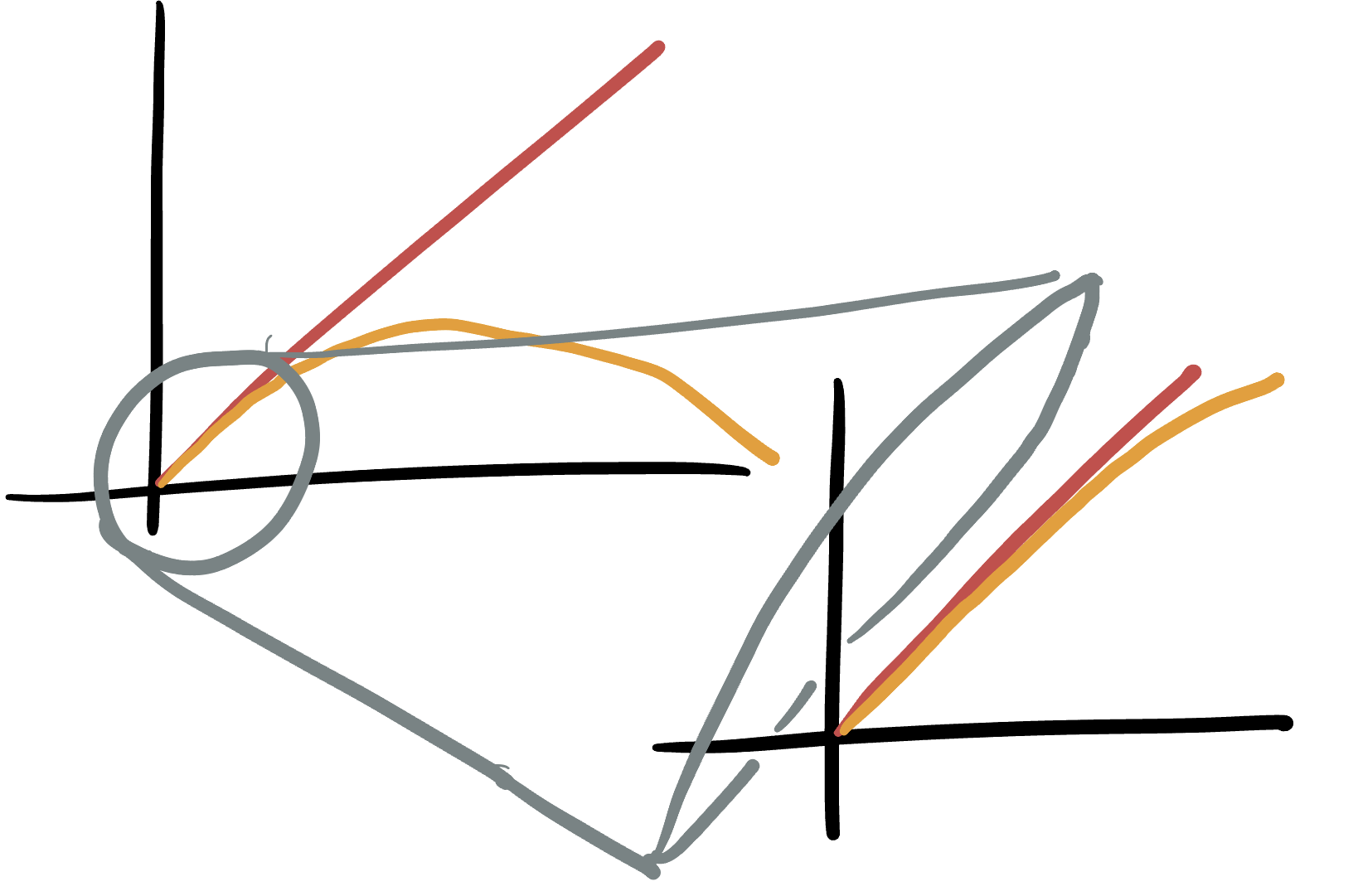
To be precise, say we have two geodesics passing through a point \(p\), which initially make an angle of \(\theta\) with respect to one another at the point of intersection. After traveling for distance \(d\) along each geodesic, how far apart are the resulting points?
The question that turns out to be most interesting mathematically isn’t the actual distance for some finite value of \(\theta\) (as the formulas can get quite messy), but rather a more infinitesimal notion, looking only at geodesics right next to our original one. Thus we want to zoom in on \(\theta\) near zero, which means we want to differentiate!
To make this precise, need a definition
Definition 19.3 Given a geodesic \(\gamma\) through some point \(p\) at \(t=0\), let \(\gamma_\theta\) be the geodesic which makes angle \(\theta\) with \(\gamma\) at \(p\).
The collection of all geodesics for \(\theta\) varying within some small interval about \(0\) is called a geodesic variation about \(\gamma\).

Definition 19.4 Given a geodesic \(\gamma\), we can measure the infinitesimal spread of nearby geodesics by taking a geodesic variation \(\gamma_\theta(t)\) and differentiating with respect to \(\theta\) at \(0\):
\[J(t)=\frac{d}{d\theta}\Bigg|_{\theta =0}\gamma_\theta(t)\]
We can work this out in Euclidean space using the distance formula: if the point is \(O\) and we set one geodesic \(\gamma\) off in direction \(\langle 1,0\rangle\), the geodesic at angle \(\theta\) starts with initial direction \(\langle \cos\theta, \sin\theta\rangle\) by definition. Since geodesics are affine functions \(p+tv\) we can write down their equations directly from this:
\[\gamma(t)=(t,0)\hspace{1cm}\gamma_\theta(t)=(t\cos\theta,t\sin\theta)\]
We see that these are spreading out linearly from one another with time, but how do we quantify this mathematically? By the infinitesimal variation!
\[\begin{align*} J(t)&= \frac{d}{d\theta}\Bigg|_{\theta=0}\gamma_\theta(t)\\ &= \frac{d}{d\theta}\Bigg|_{\theta=0}\left(t\cos\theta,t\sin\theta\right)\\ &= (-t\sin\theta,t\cos\theta)\Bigg|_{\theta=0}\\ &=(0,t) \end{align*}\]
The magnitude of the geodesic variation tells us how quickly nearby geodesics are spreading out away from \(\gamma\). Here, in flat space we see
\[\|J(t)\|=\|(0,t)\\|=t\]

But what about on the sphere? Here, we may take our geodesic to be a line of longitude, say
\[\gamma(t)=(\sin t,0,\cos t)\]
which passes through the north pole \(N=(0,0,1)\) at time zero, with initial direction
\[\gamma^\prime(0)=\frac{d}{dt}\Bigg|_{t=0}(\sin t,0,\cos t)=\langle 1,0,0\rangle\]
How do we find the geodesics through \(N\) making angle \(\theta\) with \(\gamma\)? By using isometries of course! We can rotate the sphere fixing \(N\) by angle \(\theta\) using previous work:
\[\gamma_\theta(t)=\pmat{\cos\theta & -\sin \theta & 0 \\ \sin\theta & \cos\theta &0\\ 0&0&1}\pmat{\sin t\\ 0 \\ \cos t}= \pmat{\cos\theta\sin t\\ \sin\theta\sin t\\ \cos t}\]
Now we have our geodesic variation, so all we need to do is differentiate it with respect to \(\theta\).
\[\begin{align*} J(t)&= \frac{d}{d\theta}\Bigg|_{\theta=0}\gamma_\theta(t)\\ &= \frac{d}{d\theta}\Bigg|_{\theta=0}\left(\cos\theta\sin t, \sin\theta\sin t, \cos t\right)\\ &= (-\sin\theta\sin t, \cos\theta\sin t,0)\Bigg|_{\theta=0}\\ &=(0,\sin t,0) \end{align*}\]
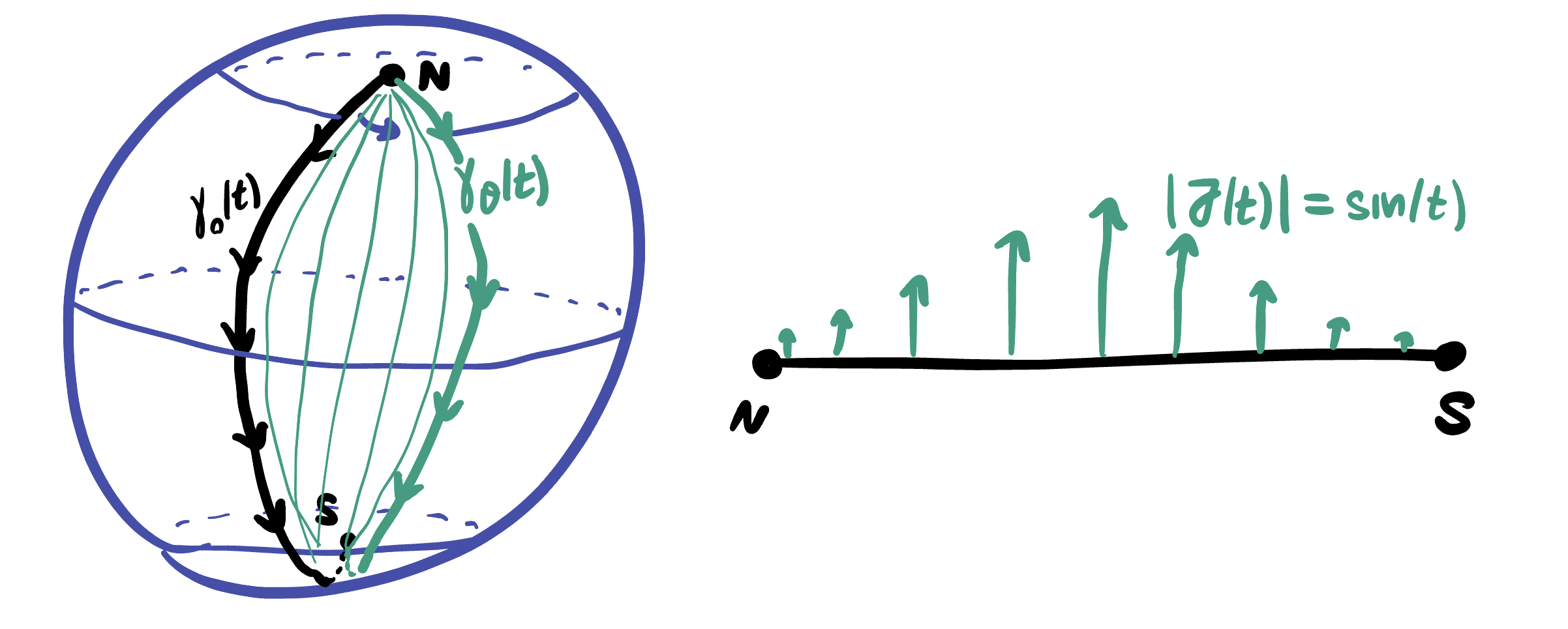
Again, the magnitude of this vector measures the rate at which nearby geodesics are diverging from one another:
\[\|J(t)\|=\|(0,\sin t,0)\|=\sin t\]
How do we interpret this? Well the sine function first grows until \(t=\tau/4\) and then begins to shrink: this means that geodesics first begin to diverge then at \(t=\tau/4\) begin to converge once more. Of course, we already knew this - because the geodesics are great circles (and we had found their explicit formulas to even compute the variation).
We’ve seen the qualitative behavior of these variations depends on the curvature: if the curvature is zero, then geodesics spread out linearly, but when its positive they oscillate sinusoidally between converging and diverging. In fact :::{#thm-jacobi-equation} Let \(J(t)\) be an infinitesimal variation along a geodesic. Then if the space we are considering has constant curvature \(\kappa\), the infinitesimal variation satisfies the differential equation
\[J^{\prime\prime}+\kappa J = 0\] :::
19.4 Spheres of Other Sizes
So far, our entire discussion has been taking place for the unit sphere, but unlike Euclidean space, there are multiple different spherical geometries: things behaved differently depending on the radius of the sphere. For each positive real number \(R\) we can define spherical geometry of radius \(R\), denoted \(\SS_R^2\), as follows.
Definition 19.5 (Spherical geometry of Radius \(R\).) Let \(\SS^2_R\) denote the set of points which are distance \(R\) from the origin in \(\EE^3\). For each point \(p\in\SS^2_R\), the tangent space \(T_p\SS^2_R\) consists of all points in \(\EE^3\) which are orthogonal to \(p\) (definition unchanged from the unit sphere), and the dot product for measuring infinitesimal lengths and angles is the standard dot product on \(\EE^3\) (also unchanged from the unit sphere).
The development of each of these spherical geometries is qualitatively very similar to that for \(\SS^2\): we can see without any change that \((x,y,z)\mapsto (x,y,-z)\) is an isometry so the equator is a geodesic, and orthogonal transformations are still isometries so all great circles are geodesics.
What changes is the quantitative details: the formulas for length area and curvature. In the next two problems, your job is to redo the calculations that I did for \(\SS^2\), for the geometry \(\SS^2_R\):
Exercise 19.4 (Circumference and area.) What is the formula for the circumference and radius of a circle of radius \(r\) on \(\SS^2_R\)?
Hint: base your circles at \(N=(0,0,R)\) and look back at our arguments from class to see what must change, and what stays the same.
Exercise 19.5 Using the definition of curvature as a limiting ratio of circumferences (Definition 4), compute the curvature of \(\SS^2_R\), and show that \[\kappa = \frac{1}{R^2}\]
Think about what this relationship says: as a sphere gets bigger in radius, it’s curvature (which measures the difference between it and the Euclidean plane) quickly decreases! That is, the bigger a sphere you have, the more difficult it is to tell apart from a plane at a point.
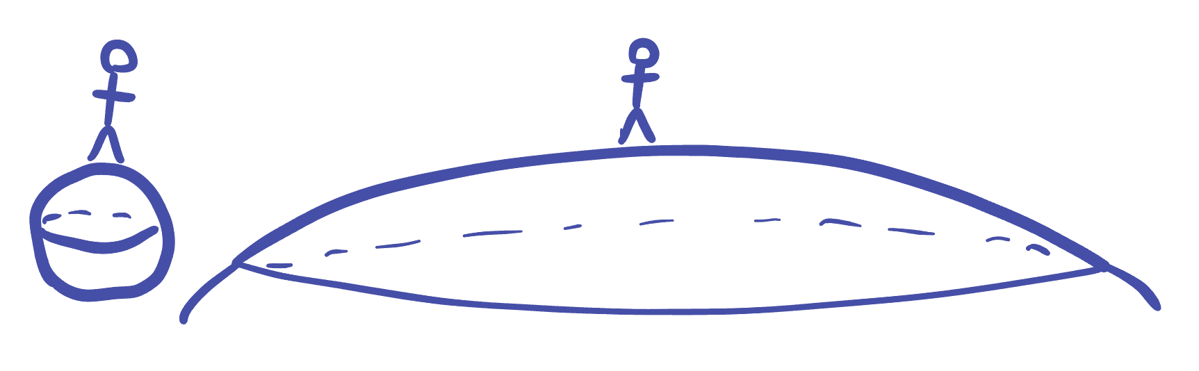
This mathematical fact has tricked an unfortunate number of people into believing that large spheres like the earth are flat. But now we know better:
Example 19.1 (Curvature of the Earth) The earth’s circumference is 40 million meters (in fact, the meter was originally defined so that the distance from the equator to the north pole was 10 million meters!). This means the radius of the earth is \[R=\frac{40,000,000}{2\pi}\approx 6,366,197\mathrm{m}\] and so the curvature of the earth is
\[\begin{align*}\kappa&=\frac{1}{R^2}\\ &=\frac{1}{40,528,473,456,935}\\&\approx 0.000000000000024674011002723\end{align*}\]
But while small, \(0.00000000000002\) is not zero, and on large enough scales this small amount of curvature actually has a big effect, on flight paths, air currents, the formation of hurricanes, etc.