14 Angles
In the geometry of Euclid, an angle was defined as being delimited by straight lines:
A plane angle is the inclination to one another of two lines in a plane which meet one another and do not lie in a straight line.
However as Greek mathematics (and beyond) turned to the problem of curves, it became necessary to also speak of curvilinear angles: that is, the angle of intersection between two curves. This was a difficult concept, as at no finite level of zoom could this be made into a “true angle”, the sides were never going to be straight.

From the modern perspective this is no issue, as zooming in on the point of intersection we may pass to the tangent space, and replace each of the curves by their linearizations. This allows us to think of angles as infinitesimal quantities based at a point.
Definition 14.1 An angle \(\alpha\) at a point \(p\in\EE^2\) is an ordered pair of tangent vectors \(\alpha=(v,w)\) based at \(p\).

The order of the tangent vectors tells us which curve is “first” and which is “second” as we trace out the angle. By convention, we will trace the angle counterclockwise from start to finish.

(Occasionally, we wish to read an angle clockwise instead: in this case we will say that it is a negative angle, whereas counterclockwise default angles are positive)
From this, we can define the angle between two curves in terms of their tangents:
Definition 14.2 Given two curves \(C_1,C_2\) which intersect at a point \(p\) in the plane, and let \(v_1\) be tangent to \(C_1\), and \(v_2\) be tangent to \(C_2\) at \(p\). Then the angle from \(C_1\) to \(C_2\) is just the pair \((v_1,v_2)\) of tangents.

14.1 Angle Measure
In all of Euclid’s elements, angles were not measured: by numbers. There was a definition of a right angle (half a straight angle), and definitions of acute and obtuse (less than, or greater than a right angle, respectively). Though they never attached a precise number, they did have the angle axioms specifying how to work with angles like they were a kind of number, however.
In our modern development we find numerical measures extremely convenient: if we can measure angles with a function, we can do calculus with angles! So we want to go further, and an actual number to each angle (which we’ll call its measure) in a way that’s compatible with the original angle axioms.
How do we construct such a number? At the moment we do not have much to work with, as our development of geometry is still in its infancy: we have essentially only constructed lines, circles and the distance function. These strict constraints essentially force a single idea for angle measure upon us:
Definition 14.3 (Angle Measure) If \(u\) and \(v\) are two unit vectors based at the same point \(p\) forming angle \(\alpha=(u,v)\), then the measure of \(\alpha\) is defined as the arclength of the unit circle centered at \(p\) that lies between them. Its denoted \[\mathrm{Angle}(\alpha)\textrm{ or }\mathrm{Angle}(u,v)\]

This is a very “basic” way of dealing with angles, as it uses so few concepts from our geometry (its close to the base definitions). Indeed, its geometric simplicity makes it exceedingly useful throughout mathematics, you’ve all met this definition before under the name radians.
Because angles are defined in terms of unit circle arclength, it will prove very convenient to have a name for the entire arclength of the unit circle. That way we can express simple angles as fractions of this, instead of as some long (probably irrational) decimal representing their arclength. We will denote the arclength of the unit circle by \(\tau\), standing for turn (as in, one full turn of the circle)
Definition 14.4 (\(\tau\)) The arclength of the unit circle is \(\tau\).

The first thing we may wish to explore is how this concept interacts with isometries.
Proposition 14.1 (Angles Measures are Invariant under Isometries) If \(\alpha\) and \(\beta\) are two angles in \(\EE^2\), and \(\phi\) is an isometry taking \(\alpha\) to \(\beta\), then the measures of \(\alpha\) and \(\beta\) are equal.
Proof. Let \(\alpha\) and \(\beta\) be two angles: so precisely \(\alpha\) is a pair of tangent vectors \(a_1,a_2\) based at a point \(p\), and \(\beta\) is a pair of tangent vectors \(b_1,b_2\) at a point \(q\).
Any isometry taking \(p\) to \(q\) takes the unit circle based at \(p\) to the unit circle based at \(q\) (since isometries preserve the distance function). And, if the isometry takes \(a_1\) to \(b_1\) as well as \(a_2\) to \(b_2\), it takes the arc of the unit circle defining \(\alpha\) to the arc defining \(\beta\).
Since isometries preserve the length of all curves, the lengths of these arcs must be the same. Thus these angles have the same measure.
Because angle measures are defined in terms of the unit circle, we can also attempt to run the above argument with a similarity \(\sigma\) instead of isometry. If the scaling factor is \(k\), the main change is that \(\sigma\) takes the unit circle to a circle of radius \(k\) (as similarities take circles to circles, Exercise 13.3). We know how similarities affect lengths - so the length of this arc is \(k\) times the original angle measure. But to correctly compute the new angle, we need to be measuring on the unit circle. So, we need to rescale it down by \(1/k\) a similarity. This then divides the length by \(k\), and overall we see the new length is identical to the original: so the angle is the same!
Corollary 14.1 (Angle Measures are Invariant Under Similarities) If \(\alpha\) and \(\beta\) are two angles in \(\EE^2\), and \(\sigma\) is an similarity taking \(\alpha\) to \(\beta\), then the measures of \(\alpha\) and \(\beta\) are equal.
Computing an angle directly from this definition is challenging, as it requires us to measure arclength. Much of the later work in this chapter will establish a beautiful means of doing this. But in certain situations, angles can be measured directly by more elementary means.
Example 14.1 (Angle between \(x\)- and \(y\)-axes) The angle from \((1,0)\) to \((0,1)\) is \(\tau/4\). To see this, recall that we have a rotation isometry fixing the origin and taking \((1,0)\) to \((0,1)\) - this was the first rotation we discovered (Example 11.1). \[R(x,y)=\pmat{0&-1\\1&0}\pmat{x\\ y}\]
Now, look what happens when you apply \(R\) multiple times in a row. This repeated composition is actually straightforward to compute, as it’s just matrix multiplication!
\[R^2=\pmat{-1&0\\0&-1}\hspace{0.5cm} R^3=\pmat{0&1\\-1&0}\hspace{0.5cm}R^4=\pmat{1&0\\0&1}\]
Looking at the last line, we see that applying \(R\) four times in a row results in the identity matrix - or the transformation that does nothing to the inputs! That is, after four rotations we are back to exactly where we have started.

Because isometries preserve angles (Proposition 14.1), we see that our isometry \(R\) has covered the entire unit circle in exactly four copies of our original angle. Thus, the angle measure must be \(1/4\) of a circle: \[\theta = \frac{\tau}{4}\]
(This example tells us our first rotation angle: the matrix \(\smat{0&-1\\1&0}\) rotates the plane by a quarter turn or \(\tau/4\)! This will be a very useful fact, and we will even put it to use shortly, in Proposition 14.3 where we find the derivative of \(\sin\) and \(\cos\). )
Exercise 14.1 (Angle Measure of Equilateral Triangle) Show the angle measure of an equilateral triangle is \(\tau/6\), in a similar method to the example above.
To start, draw an equilateral triangle with unit side length, and one side along the \(x\)-axis. In Exercise 23, you found that the third vertex of this must lie at \(p=(1/2,\sqrt{3}/2)\). From this, we can write down a rotation isometry (Theorem 11.4) taking \((1,0)\) to \(p\). The angle this rotates by is exactly the angle our triangle’s sides make at the origin.
Show that if you apply this rotation three times, you get negative the identity matrix. Use this to help you figure out how many times you have to apply it before you get back to the identity! Then use that isometries preserve angles, and the circumference of the unit circle is \(\tau\) to deduce the angle you are after.
Proposition 14.1 and Example 14.1, Exercise 14.1 showcase two essential properties of the angle measure which stem from the fact that we defined it as a length: its invariant under isometries, and easy to subdivide. In fact, these are precisely the angle axioms of the greeks!
Example 14.2 (Proving the “Angle Axioms”) Now that we have a definiiton of angle measure in terms of more primitive quantities (vectors, lengths, circles), we can prove that this measure satisfies the greek axioms.
Congruent Angles have Equal Measures Since two angles are congruent if there is an isometry taking one to the other, and the measure of an angle is invariant under isometries, congruent angles have the same measure.
Subdividing an Angle If we divide an angle \(\theta\) into two angles \(\theta_1,\theta_2\) by a line, then \(\theta = \theta_1+\theta_2\). This follows directly from a property of integrals! Since an angle is a length, and a length is an integral we can use the property \(\int_a^b fdx=\int_a^c fdx+\int_c^bfdx\) to prove \(\theta = \theta_1+\theta_2\).
14.2 Working With Angles
We now turn to the problem of actually computing things with the angle measure. To do so, it’s helpful to choose a “basepoint” on the circle to take first measurements from - here we’ll pick \((1,0)\).
Definition 14.5 (Arclength Function) The arclength function takes in a point on the unit circle \((x,y)\), and measures the arclength \(\theta\) from \((1,0)\) to this point. \[\Theta(x,y)=\textrm{arclength from $(1,0)$ to $(x,y)$}\]
In this section, we will study in detail expressions for this function, and its inverse.
14.2.1 Arc- Sine and Cosine
Because the points of the unit circle satisfy \(x^2+y^2=1\), if we know the sign of \(x,y\) (which half of the circle the point lives in) we can fully reconstruct the point from a single coordinate: either \((x,\pm\sqrt{1-x^2})\) or \((\sqrt{1-y^2},y)\). Thus, so long as we remember the correct sign of the second coordinate of interest, the arclength function is essentially a function of one variable. We could take just the \(x\) or \(y\) coordinate of a point on the circle and define a function like \(\Theta(x)\) which would measure the arclength to \((x,\sqrt{1-x^2})\), or \(\Theta(y)\) if we expressed the point \((\sqrt{1-y^2},y)\). However, we do not need to invent our own notation for these arclength functions of one variable, they are already well known to us from trigonometry!
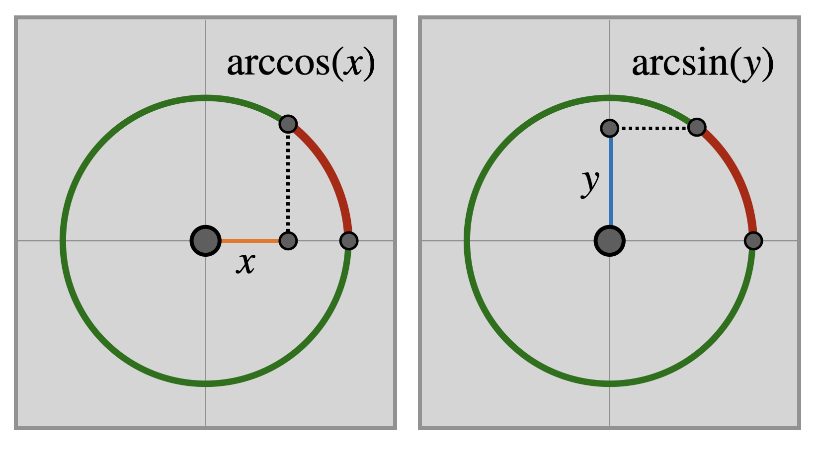
Definition 14.6 (Arc Functions: Inverse Trigonometry) The functions \(\arccos\) and \(\arcsin\) compute the arclength along the unit circle from \((1,0)\) to the point \((x,y)\) as \[\arccos(x)=\textrm{arclength from $(1,0)$ to $(x,\sqrt{1-x^2})$}\] \[\arcsin(y)=\textrm{arclength from $(1,0)$ to $(\sqrt{1-y^2},y)$}\]
This of course does nothing to help us compute these functions: we’ve just given a name to them. In fact, we can compute only very few values from first principles:
Example 14.3 (“Unit Circle Values” for Arc Functions) -The point \((1,0)\) lies at arclength zero from \((1,0)\)…as they are the same point! Thus, \[\arccos(1)=0\hspace{1cm}\arcsin(0)=0\]
The point \((0,1)\) lies a quarter of the way around the circle (Example 14.1), so has arclength \(\tau/4\). Thus we see \[\arccos(0)=\tau/4\hspace{1cm}\arcsin(1)=\tau/4\]
Looking at Exercise 14.1 where we found the angle of a unit equilateral triangle with sides vertices \((0,0),(1,0)\) and \((1/2,\sqrt{3}/2)\) to be \(\tau/6\), we see \[\arccos(1/2)=\tau/6\hspace{1cm}\arcsin(\sqrt{3}/2)=\tau/6\]
What we need is some sort of concrete expression telling us how to compute \(\arccos(x)\) (or arcsin) for arbitrary values of \(x\). And here we can make essential use of our definition of angle as a length, and length as an integral! Unpacking it all gives directly an integral formula to compute \(\arccos(x)\):
Proposition 14.2 (Integral Representation of \(\arccos(x)\)) For \(x\in [-1,1]\), the arccosine function can be computed via an integral \[\arccos(x)=\int_x^1 \frac{1}{\sqrt{1-t^2}}dt\]
Proof. By definition, the \(\arccos(x)\) is the length of circle between \(x\) and \(1\). Since \(x^2+y^2=1\), we may parameterize the top half of the circle using \(x\) as the parameter by \[c(t)=(t,\sqrt{1-t^2})\] Thus, as lengths are integrals, we can already give an expression for \(\arccos(x)\): \[\arccos(x)=\int_x^1 \|c^\prime(t)\|dt\] To be useful, we must expand out the integrand here, and compute \(\|c^\prime\|\):
\[c^\prime(t)=\left(1,\frac{-t}{\sqrt{1-t^2}}\right)\]
And then, we must find its norm: \[\begin{align*} \|c^\prime(t)\|&=\sqrt{1+\left(\frac{-t}{\sqrt{1-t^2}}\right)^2}\\ &=\sqrt{1+\frac{t^2}{1-t^2}}\\ &=\sqrt{\frac{1}{1-t^2}} \end{align*}\]
Thus, we have an integral representation of the arccosine!
\[\arccos(x)=\int_x^1\frac{1}{\sqrt{1-t^2}}dt\]
If we start at \(x=-1\) and go to \(x=1\), this curve traces out exactly half of the unit circle (the top half). Thus, twice this value is an integral representing our fundamental constant \(\tau\):
Corollary 14.2 (Defining \(\tau\):) \[\tau = \int_{-1}^1\frac{2}{\sqrt{1-x^2}}dx\]
Exercise 14.2 Complete an analogous arugment to the above to show \[\arcsin(y)=\int_0^y\frac{1}{\sqrt{1-t^2}}dt\]
These formulas, via the fundamental theorem of calculus, tell us the derivative of \(\arcsin\) and \(\arccos\) as well!
Corollary 14.3 (Differentiating the Arc Functions) The derivative of the arc functions are \[\frac{d}{dx}\arccos(x)=\frac{-1}{\sqrt{1-x^2}}\] \[\frac{d}{dy}\arcsin(y)=\frac{1}{\sqrt{1-y^2}}\]
Proof. Each of these is an immediate application of the fundamental theorem of calculus: but there’s a small subtlety in how we usually apply this theorem to the first, so we will start with \(\arcsin\).
The fundamental theorem says that \(\frac{d}{dx}\int_a^x f(t)dt=f(x)\), so we immediately get \[\frac{d}{dy}\arcsin(y)=\frac{d}{dy}\int_0^y \frac{1}{\sqrt{1-t^2}}dt=\frac{1}{\sqrt{1-y^2}}\]
The difficulty with arccosine is that in the way we have it written, the variable \(x\) is the lower bound of the integral. To prepare this expression for an application of the fundamental theroem, we must first switch the bounds, which negates the integral. Thus
\[\frac{d}{dx}\arccos(x)=\frac{d}{dx}\int_1^x \frac{-1}{\sqrt{1-t^2}}dt=\frac{-1}{\sqrt{1-x^2}}\]
This is where the negative sign in the derivative of arccosine comes from: I have to remind myself of this every time I teach calculus 1.
14.2.2 Sine and Cosine
Now that we have the functions that measure arclength, its natural to ask about their inverses: if we know the arclength from \((1,0)\) to a point, can we recover the coordinates of the point?
Definition 14.7 (Sine and Cosine) Let \(p\) be the point on the unit circle centered at \(O\) which lies at a distance of \(\theta\) in arclength from \((1,0)\). Then we define \(\cos(\theta)\) as the \(x\)-coordinate of \(p\), and \(\sin\theta\) as the \(y\)-coordinate of \(p\).

Example 14.4 At \(\theta=0\), we have moved no distance along the circle from \((1,0)\), so we are still at \((1,0)\). Thus \[\cos(0)=1\hspace{1cm}\sin(0)=0\]
(Because sine and cosine are defined as lengths, which are invariant under isometries, we see that we could equally well define these functions from a unit circle centered at any point in \(\EE^2\). After the chapter on symmetry, we will see that we can further generalize to base them on any circle whatsoever.)
Beyond this, the definition doesn’t give us any means at all of calculating the value of \(\cos\) or \(\sin\): we’re going to need to do some more work to actually figure out what these functions are! For their inverses, the secret was unlocked by integration, and so it makes sense that here we must do the opposite, and look to differentiation for help!
Proposition 14.3 (Differentiating Sine & Cosine) The derivatives of \(\sin(\theta)\) and \(\cos(\theta)\) are as follows: \[\frac{d}{d\theta}\sin\theta = \cos \theta\hspace{1cm}\frac{d}{d\theta}\cos\theta = -\sin\theta\]
There are many beautiful geometric arguments for computing the derivative of \(\sin\theta\) and \(\cos\theta\), involving shrinking triangles and side ratios. Below is a different style argument, which fits well with the calculus-first perspective of our course. We use the fact that the derivative gives the tangent line to figure out what it must be!
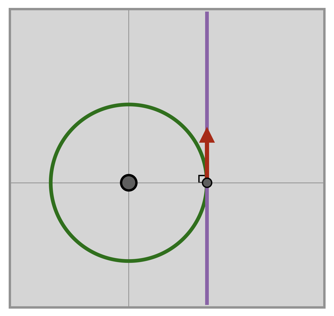
Proof. Let \(C\) be the unit circle centered at \((0,0)\), and \(\gamma(t)=(\cos(\theta),\sin(\theta))\) be the arclength parameterization defined above. Because \(\gamma\) traces out the circle with respect to arclength, its derivative with respect to arclength is unit length, by definition.
We start by finding the derivative at \((1,0)\). As the radius of the circle is \(1\) and the \(x\)-coordinate at \(\gamma(0)=(1,0)\) equal to \(1\), we are at a maximum value of the \(x\)-coordinate. Differential calculus (Fermat’s Theorem) tells us that at a maximum, the derivative is zero. So, \(x^\prime=0\) at \((1,0)\). But \(y^\prime\) cannot also be zero here: as \(y\) is increasing as we trace out the circle, differential calculus (a corollary of the Mean Value Theorem) tells us that \(y^\prime(0)\) is positive. But now the fact that \(\|\gamma^\prime(0)\|=1\) uniquely singles out a vector: \[\gamma^\prime(0)=\langle 0,1\rangle_{(1,0)}\]
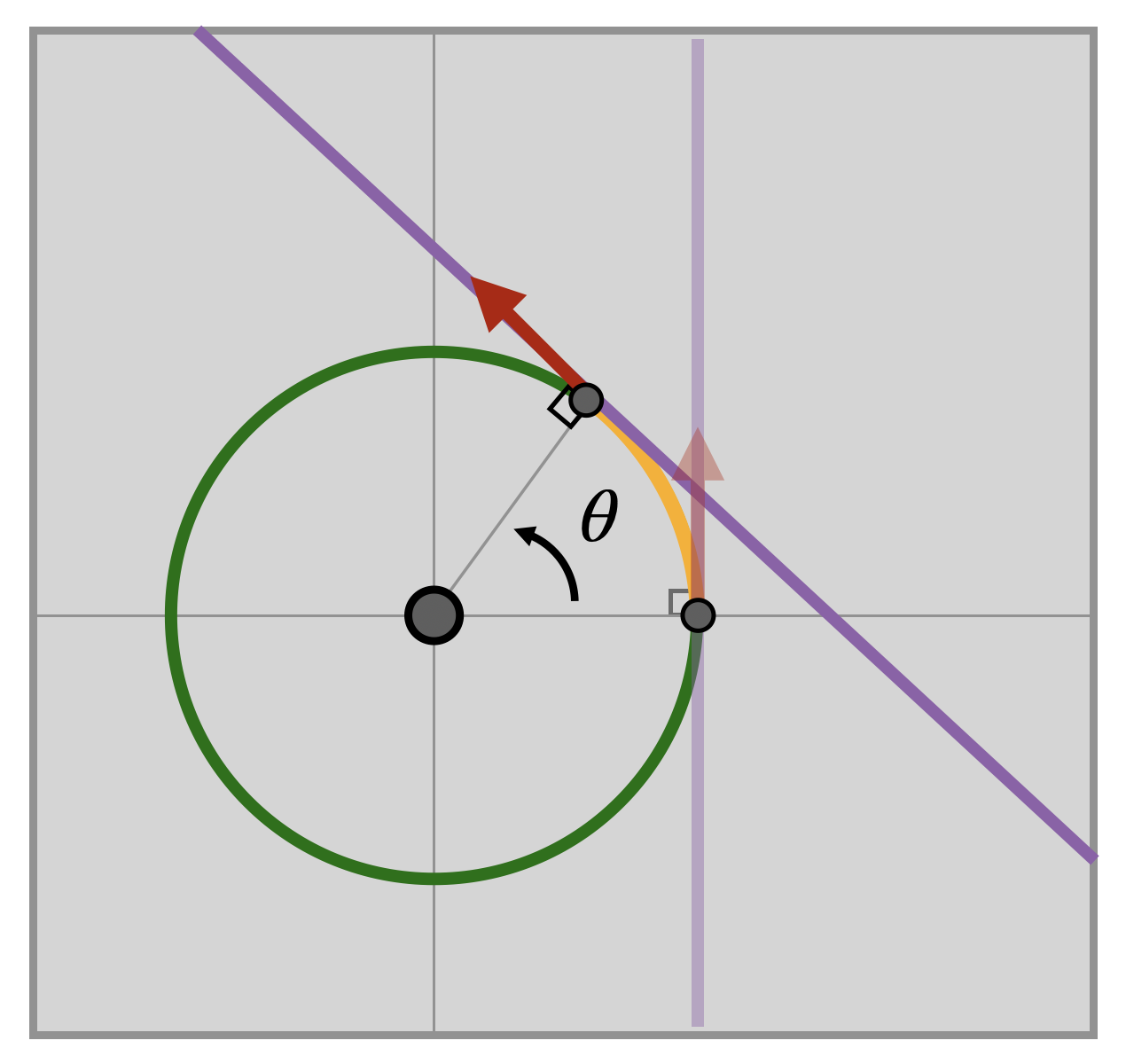
This is actually all the differentiation we have to do! The rest of the argument amounts to a clever use of isometries. Choose a point \(q=\gamma(\theta)=(\cos(\theta),\sin(\theta))\) on the circle, where we wish to compute the tangent vector. Now create an isometry \(\phi\) taking \((1,0)\) to \(q\). Since rotations about the center preserve circles (Proposition 13.1), the curve \(\phi\circ\gamma\) also traces out the unit circle. Thus, if we find the tangent to \(\phi\circ\gamma\) at \(q\) we’ll have found the tangent to the circle at \(q\)!
At \((1,0)\), we saw the tangent vector was a \(\tau/4\) rotation from the vector connecting its basepoint to the origin. Since isometries preserve angles (Proposition 14.1), it must also be true that the tangent vector at \(q\) is a \(\tau/4\) rotation of \(q-O=\langle \cos \theta,\sin \theta\rangle_q\). And we know how to rotate a vector by \(\tau/4\): switch its coordinates and negate the first (Example 11.1)! \[\langle \cos \theta,\sin \theta\rangle_q \mapsto \langle -\sin \theta,\cos \theta\rangle_q\]
Since the tangent vector to the the circle at \(q\) is the derivative of \(\gamma\) at \(\theta\), this tells us exactly what we were after:
\[\begin{align*} \gamma^\prime(\theta)&=\langle(\cos \theta)^\prime,(\sin \theta)^\prime \rangle\\ & = \langle -\sin \theta,\cos \theta\rangle \end{align*}\]
Remark 14.1. An alternative to the first step of this proof is to consider that the circle is sent to itself under the isometry \(\phi(x,y)=(x,-y)\). This map fixes the point \((1,0)\), and so it must send the tangent line at \((1,0)\) to itself. But as \(\phi\) is linear, its derivative is itself, so it applies to tangent vectors also as \(\phi(v_1,v_2)=\langle v_1,-v_2\rangle\). Thus, whatever the tangent vector at \((1,0)\) is, it must be a vector such that \(\langle v_1,v_2\rangle\) is parallel to \(\langle v_1,-v_2\rangle\). This forces \(v_1=0\), and then unit length forces \(\langle 0,\pm 1\rangle\).
Exercise 14.3 Because of our hard work with the arc functions already, we have an alternative approach to differentiating sine and cosine, using purely the rules of single variable calculus!
- Explain why from the definition of \(\sin,\cos\) we know that \(\sin^2\theta+\cos^2\theta =1\)
- Use the technique for differentiating an inverse () to differentiate \(\sin\) as the inverse function of \(\arcsin\), whose derivative we know.
- Combine these two facts to simplify the result you got, and show \(\sin(\theta)^\prime=\cos(\theta)\).
- Repeat similar reasoning to show \(\cos(\theta)^\prime=-\sin(\theta)\).
Remark 14.2. An alternative second part to this proof is just to write down the matrix: we know the rotation taking \((1,0)\) to \((p_1,p_2)\) is \(\smat{q_1 &-q_2\\ q_2 &q_1}\), so for \(q=(\cos t, \sin t)\) its \(\smat{\cos t &-\sin t\\ \sin t & \cos t}\). This is linear so we can apply it to both points and vectors: applying to the tangent vector \(\langle 0,1\rangle_{(1,0)}\) just reads off the second column! Thus the tangent vector at \(q\) is \(\langle -\sin\theta, \cos\theta\rangle_q\).
Believe it or not - we already have enough information to completely understand the sine and cosine functions! Since they are each other’s derivatives, and we know both values at zero, we can directly write down their series expansions!
Proposition 14.4 (Series Expansions of Cos) The series expansion of the cosine function is \[\begin{align*}\cos\theta &= \sum_{n=0}^\infty\frac{(-1)^n}{(2n)!}\theta^{2n}\\ &= 1-\frac{\theta^2}{2}+\frac{\theta^4}{4!}-\frac{\theta^6}{6!}+\frac{\theta^8}{8!}-\frac{\theta^{10}}{10!}-\cdots \end{align*}\]
Proof. We first build what the series ought to be (assuming it exists), and then we prove that our candidate actually converges! Assume that \(\cos\theta =a_0+a_1\theta+a_2\theta^2+\cdots\) for some coefficients \(a_n\). Evaluating this at \(\theta =0\) we see \[\cos 0 = a_0 + a_1\cdot 0 + a_2\cdot 0^2+\cdots=a_0\] Since we know \(\cos 0 =1\) this says \(a_0=1\), and we have determined the first term in the series:
\[\cos\theta = 1 + a_1\theta +a_2\theta^2+a_3\theta^3+a_4\theta^4\cdots\]
So now we move on to try and compute \(a_1\). Taking the derivative of this series gives
\[(\cos \theta)^\prime = a_1+2a_2\theta +3a_3\theta^2+\cdots\] And again - every term except the first has a \(\theta\) in it, so evaluating both sides at zero gives us \(a_1\). Using that cosine’s derivative is \(-\sin\theta\), we get \(-\sin(0)=0=a_1\), so \(a_1\) is zero.
\[\cos\theta = 1 + 0\theta +a_2\theta^2+a_3\theta^3+a_4\theta^4+\cdots\]
Moving on to \(a_2\), we must differentiate one more time to get the term with \(a_2\) to have no \(\theta\)s in it:
\[(\cos\theta)^{\prime\prime}=2a_2+3\cdot 2a_3 \theta+ 4\cdot 3a_4\theta^2+\cdots\]
Since \((\cos\theta)^\prime = -\sin\theta\) and \((-\sin\theta)^\prime =-\cos\theta\), this series is equal to \(-\cos\theta\)! And evaluating at \(0\) gives \(-1\). Thus \(2a_2=-1\) so \(a_2=-\tfrac{1}{2}\).
\[\cos\theta = 1 + 0\theta -\frac{1}{2}\theta^2+a_3\theta^3+a_4\theta^4+\cdots\]
Continuing to \(a_3\) differentiating the left side once more gives \(\sin\theta\) which evaluates to zero, and the right results in a function with constant term \(3\cdot 2a_3\): thus \(a_3\) is zero.
\[\cos\theta = 1 + 0\theta -\frac{1}{2}\theta^2+0\theta^3+\cdots\]
Differentiating once more, the left side has returned to \(\cos\theta\) and the right now has constant term \(4\cdot 3\cdot 2 a_4\): thus \(a_4=1/4!\).
\[\cos\theta = 1 + 0\theta -\frac{1}{2}\theta^2+0\theta^3+\frac{1}{4!}\theta^4+\cdots\]
After repeating the process four times, we’ve cycled back around to the same function \(\cos\theta\)-that we started with! And so continuing, the same pattern in derivatives, \(1,0,-1,0\cdots\) will continue to repeat. This tells us every odd term will be zero in our series, and the even terms will have alternating signs:
\[\cos\theta = 1-\frac{1}{2!}\theta^2+\frac{1}{4!}\theta^4-\frac{1}{6!}\theta^6+\frac{1}{8!}\theta^8-\cdots\]
Thus *if \(\cos\theta\) can be written as a series at all - it must be this one! We only have left to confirm that this series actually converges (and thus, by Taylor’s theorem, equals the cosine).
Exercise 14.4 Prove that the series for \(\cos\) converge for all real inputs: that is, that their radius of convergence is \(\infty\). Hint: review the ratio test!
Exercise 14.5 (Series Expansion of Sin) Run an analogous argument to the above to show \[\sin \theta = \sum_{n=0}^\infty \frac{(-1)^n}{(2n+1)!}\theta^{2n+1}\]
14.3 The Dot Product
Having explicitly computable formulas for \(\arccos\) and \(\arcsin\) (even though they are via integral expressions, and probably need to be evaluated numerically as Riemann sums) lets us act as though knowing the cosine or sine of an angle is just as good as knowing the angle itself.
Example 14.5 What is the angle between \((1,0)\) and \((1,2)\)?
We figure out where the second vector intersects the unit circle by dividing by its magnitude: \((1/\sqrt{5},2/\sqrt{5})\). Now we know by definition that whatever the arclength \(\theta\) is, its cosine is the first coordinate. And being able to compute arccosines, we immediately get \[\cos\theta=\frac{1}{\sqrt{5}}\implies\theta = 1.10714\mathrm{rad}\]
Our goal in this section is to generalize the example above into a universal tool, that lets us compute the measure of any angle in the Euclidean plane using a simple tool from linear algebra: the dot product.
Definition 14.8 The dot product of \(u=\langle u_1,u_2\rangle\) and \(v=\langle v_1,v_2\rangle\) is \[u\cdot v = u_1v_1+u_2v_2\]
We can already directly compute the angle a unit vector \(v=\langle v_1,v_2\rangle\) makes with \(\langle 1,0\rangle\): in this situation \(v_1=\cos\theta\) by definition, or \(\langle 1,0\rangle\cdot v=\cos\theta\). But if \(u\) and \(v\) are two unit vectors based at \(0\), how can we analogously compute the angle they form?
Theorem 14.1 (Dot Product Measures Arclength) If \(u,v\) are unit vectors based at \(p\in\EE^2\) making angle \(\theta\), then \[u\cdot v = \cos\theta\]
Proof. Let \(u,v\) denote an angle based at \(p\).The idea is to use isometries to reduce this to the case we already understand! First, let \(\phi\) be a translation isometry taking \(p\) to \(0\). Since the derivative of a translation is the identity, this takes \(u\) and \(v\) to the origin without changing their coordinates. And, since isometries preserve angle measures, we know the angle \(\theta\) between \(u_p,v_p\) is the same as the angle between \(u_o,v_o\).
Now let \(R\) be a rotation about \(O\) taking \(u_o\) to \(\langle 1,0\rangle_o\). Since angles are invariant under isometry, the angle measure between \(u_o\) and \(v_o\) is the same as between \(Ru_o\) and \(Rv_o\). But since \(Ru_o=\langle 1,0\rangle_o\), we know
\[\cos\theta = \textrm{first component of }Rv\]
Thus, all we need to do is compute the matrix \(R\), apply it to \(v\), and read off the first component of the resulting vector! We know from Theorem 11.4 how to create a rotation fixing \(O\) that takes \(\langle 1,0\rangle_o\) to \(u_o\) is \(\smat{u_1 &-u_2\\u_2 &u_1}\). The transformation \(R\) we need is the inverse of this:
\[R=\pmat{u_1 & -u_2\\u_2 & u_1}^{-1}=\pmat{u_1 & u_2\\ -u_2 & u_1} \]
Now we apply this to \(u\) and \(v\) to get our new vectors: applying to \(u\) gives \(\langle 1,0\rangle\) (check this!) and applying to \(v\) gives
\[Rv=\pmat{u_1 & u_2\\ -u_2 & u_1}\pmat{v_1\\ v_2}=\pmat{u_1v_1+u_2v_2 \\ -u_2v_1+u_1v_2}\]
The first component here is exactly \(u\cdot v = u_1v_1+u_2v_2\). Thus we are done!
The above applies explicitly to unit vectors, as we used the rotation constructed in Theorem 11.4 to requires a unit vector to send \(\langle 1, 0\rangle\) to. However, this is easily modified to measure the angle between non-unit vectors: just divide by their magnitudes first!
Corollary 14.4 The measure \(\theta\) of the angle between any two vectors \(u,v\) based at a point \(p\in\EE^2\) is related to the dot product via \[u\cdot v = \|u\|\|v\|\cos\theta\]
Proof. Let \(u,v\) be any two vectors based at \(p\). Then \(u/\|u\|\) and \(v/\|v\|\) are two unit vectors based at \(p\), and the angle between a pair of vectors is independent of their lengths (as its defined as an arclength along the unit circle no matter what). Using Theorem 14.1 we find the angle between these unit vectors: \[\frac{u}{\|u\|}\cdot \frac{v}{\|v\|}=\cos\theta\] Multiplying across by the product of the magnitudes gives the claimed result.
Exercise 14.6 Prove that rectangles exist, using all of our new tools! (Ie write down what you know to be a rectangle, explain why each side is a line segment, parameterize it to find the tangent vectors at the vertices, and use the dot product to confirm that they are all right angles).
14.3.1 Trigonometric Identities
Using very similar reasoning to the above proposition relating angles to dot products, we can leverage our knowledge of rotations to efficiently discover trigonometric identities! We consider here the angle sum identities for sine and cosine.
Theorem 14.2 (Angle Sum Identites) Let \(\alpha,\beta\) be lengths of arc (equivalently, measures of angles) and \(\alpha+\beta\) the angle formed by concatenating the two lengths. Then
\[\sin(\alpha+\beta)=\sin\alpha\cos\beta+\cos\alpha\sin\beta\] \[\cos(\alpha+\beta)=\cos\alpha\cos\beta-\sin\alpha\sin\beta\]
Proof. Let \(v=\langle v_1,v_2\rangle\) be a vector that makes angle \(\alpha\) with \(\langle 0,1\rangle\), and \(u=\langle u_1,u_2\rangle\) be a vector that makes angle \(\beta\) with \(\langle 1,0\rangle\).

Now let \(R\) be an isometry that rotates \(\langle 1,0\rangle\) to \(u\). Since isometries preserve length, this takes the segment of the unit circle between \(\langle 1,0\rangle\) and \(v\) to a segment of the same length between \(u\) and \(Rv\). So, now the total length of arc from \(\langle 1,0\rangle\) to \(Rv\) is \(\alpha+\beta\)
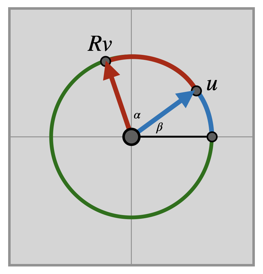
Thus, the \(x\) and \(y\) coordinates of \(Rv\) are the cosine and sine of \(\alpha+\beta\) respectively. Writing down the rotation \(R\) (via Theorem 11.4) we see \[Rv = \pmat{u_1 &-u_2\\u_2&u_1}\pmat{v_1\\ v_2}=\pmat{u_1v_1-u_2v_2\\ u_1v_1+u_1v_2}=\pmat{\cos(\alpha+\beta)\\\sin(\alpha+\beta)}\]
Finally - since \(v\) makes an angle of \(\alpha\) wtih \(\langle 1,0\rangle\) and \(u\) makes an angle of \(\beta\), we know by definition that their coordinates are \(v=(\cos\alpha,\sin\alpha)\) and \(u=(\cos\beta,\sin\beta)\). Substituting these in gives the identities we seek.
Analogously, we have the angle difference identities, which differ only in the choice of \(\pm\) signs.
Theorem 14.3 (Angle Difference Identities) \[\sin(\alpha-\beta)=\sin\alpha\cos\beta-\cos\alpha\sin\beta\] \[\cos(\alpha-\beta)=\cos\alpha\cos\beta+\sin\alpha\sin\beta\]
Exercise 14.7 Prove Theorem 14.3 similarly to how we proved Theorem 14.2 (you may need an inverse matrix!).
From these we can deduce the double angle formulas by setting both \(\alpha\) and \(\beta\) equal to the same angle \(\theta\) in the addition formula
Corollary 14.5 (Double Angle Identities) \[\cos(2\theta)=\cos^2\theta -\sin^2\theta\hspace{1cm} \sin(2\theta)=2\sin\theta\cos\theta\]
And the half angle formulas by algebraic manipulation of the above:
Corollary 14.6 (Half Angle Identities) \[\cos\left(\frac{\theta}{2}\right)=\sqrt{\frac{1+\cos\theta}{2}}\hspace{1cm}\sin\left(\frac{\theta}{2}\right)=\sqrt{\frac{1-\cos\theta}{2}}\]
Proof. We prove the cosine identity here, and leave the other as an exercise. Starting from the double angle identity for cosine, and the fact that \(\sin^2(x)+\cos^2(x)=1\), we can do the following algebra: \[\begin{align*} \cos(2x)&=\cos^2(x)-\sin^2(x)\\ &=\cos^2(x)-(1-\cos^2(x))\\ &= 2\cos^2(x)-1 \end{align*}\]
Now, we just solve for \(\cos(x)\) in terms of \(\cos(2x)\):
\[2\cos^2(x)=1+\cos(2x)\,\implies\, \cos(x)=\sqrt{\frac{1+\cos(2x)}{2}}\]
This lets us compute the cosine of an angle in terms of twice that angle! Replace \(2x\) with \(\theta\) to get the form above.
Exercise 14.8 Prove the half-angle identity for \(\sin x\).
These formulas are actually quite useful in practice, to find exact values of the trigonometric functions at different angles, given only the few angles we have computed explicitly (\(\tau/4\), for a square, and \(\tau/6\) from an equilateral triangle).
Example 14.6 (The exact value of \(\sin(\tau/24)\)) There are several ways we could approach this: one is to start with \(\tau/6\) and bisect twice. Another is to notice that \[\frac{\tau}{24}-\frac{\tau}{6}-\frac{\tau}{8}\] and use the angle subtraction identity. We will do the latter here, and below in the discussion of Archimedes cover the repeated bisection approach.
Theorem 14.3 tells us that
\[\sin\frac{\tau}{24}=\sin\frac{\tau}{6}\cos\frac{\tau}{8}-\cos\frac{\tau}{6}\sin\frac{\tau}{8}\]
We’ve successfully reduced the problem to knowing the sine and cosine of the larger angles \(\tau/6\) and \(\tau/8\). These are both do-able by hand: for \(\tau/8\) we could either note that this is half a right angle so lies along the line \(y=x\), and solve for the point \((x,x)\) on the unit circle getting \[\sin\frac{\tau}{8}=\sqrt{2}{2}\hspace{1cm}\cos\frac{\tau}{8}=\frac{\sqrt{2}}{2}\] Or, we could have started with the right angle directly and applied bisection. For \(\tau/6\), we may use Exercise 14.1 to see \[\sin\frac{\tau}{6}=\frac{\sqrt{3}}{2}\hspace{1cm}\cos\frac{\tau}{6}=\frac{1}{2}\]
The rest is just algebra:
\[\begin{align*}\sin\frac{\tau}{24}&=\frac{\sqrt{3}}{2}\frac{\sqrt{2}}{2}-\frac{1}{2}\frac{\sqrt{2}}{2}\\ &= \frac{\sqrt{2}}{4}\left(\sqrt{3}-1\right)\\ &\approx 0.258819 \end{align*}\]
14.3.1.1 The Measurement of the Circle
The half angle identities played a crucial role in Archimedes’ ability to compute the perimeter of \(n\)-gons in his paper The Measurement of the Circle. Indeed, to calculate the circumference of an inscribed \(n\)-gon, its enough to be able to find \(\sin\tau/(2n)\):

By repeatedly bisecting the sides, we can start with something we can directly compute - like a triangle, and repeatedly bisect to compute larger and larger \(n\)-gons.

Example 14.7 (From Triangle to Hexagon to 12-Gon) Start by inscribing an equilateral triangle in the circle. The angle formed by each side at the center is \(\tau/3\), and so bisecting a side gives an angle of \(\tau/6\) - the same as the angle of the equilateral triangle itself! We know the sine and cosine of this angle from Exercise 14.1: \[\cos\frac{\tau}{6}=\frac{1}{2}\hspace{1cm}\sin\frac{\tau}{6}=\frac{\sqrt{3}}{2}\]
Thus, the length of one side is \(2\cdot \frac{\sqrt{3}}{2}=\sqrt{3}\), and the circumference is \(3\sqrt{3}\approx 5.1961524\).
Doubling the side number to get to the hexagon requires we compute \(\sin\frac{\tau}{12}\), which we do via-half angle: \[\sin\frac{\tau}{12}=\sqrt{\frac{1-\cos\frac\tau 6}{2}}=\sqrt{\frac{1}{4}}=\frac{1}{2}\]
Thus, the side length here is \(1\) and the circumference is six times that, or \(6\). Doubling once more we now need to compute \(\sin\frac{\tau}{24}\) via the half-angle identity:
\[\sin\frac{\tau}{24}=\sqrt{\frac{1-\cos\frac{\tau}{12}}{2}}\] Unfortunately - we do not know \(\cos\tau/12\) yet: but we can find it! Since \(\cos^2(x)+\sin^2(x)=1\) we may use the fact that we know \(\sin\frac{\tau}{12}=\frac{1}{2}\) to calculate it:
\[\cos\frac{\tau}{12}=\sqrt{1-\left(\frac{1}{2}\right)^2}=\frac{\sqrt{3}}{2}\]
Plugging this back in, we get what we are after:
\[\sin\frac{\tau}{24}=\sqrt{\frac{1-\frac{\sqrt{3}}{2}}{2}}=\frac{\sqrt{2-\sqrt{3}}}{2}\approx 0.258819\]
Thus the length of one side of the \(12\)-gon is \(\sqrt{2-\sqrt{3}}\), and its total perimeter is \(12\sqrt{2-\sqrt{3}}\approx6.21165\)
(Note: using a different set of identities we get a different looking expression for our final answer here: a square root of a square root! But - its exactly the same value. Can you do some algebra to prove it?)
Exercise 14.9 Continue to bisections until you can compute \(\sin(\tau/(2\cdot 96))\). What is the perimeter of the regular \(96\)-gon (use a computer to get a decimal approximation, after your exact answer).
Explain how we know that this is provably an underestimate of the true length, using the definition of line segments.
Be brave - and go beyond Archimedes! Compute the circumference of the 192-gon.
Exercise 14.10 In the 400s CE, Chinese mathematician Zu Chongzi continued this process until he reached the \(24,576\)-gon, and found (in our modern notation) that \(3.1415926 < \pi < 3.1415927\). How many times did he bisect the original equilateral triangle?
Exercise 14.11 Can you use trigonometry to find the perimeter of circumscribed \(n\)-gons as well? This would give you an upper bound to \(\tau\), to complement the lower bound found from inscribed ones.

14.4 Euclid’s Axioms 4 & 5
The final two of Euclid’s postulates mention angles. Now that we have constructed them within our new foundations, we can finally attempt to prove these two!
The fourth postulate states all right angles are equal. Of course, by equal Euclid meant congruent as he often did. In order to be precise, it helps to spell everything out a bit better.
Proposition 14.5 (Euclids’ Postulate 4) Given the following two configurations: - A point \(p\), and two orthogonal unit vectors \(u_p,v_p\) based at \(p\) - A point \(q\), and two orthogonal unit vectors \(a_q,b_q\) based at \(q\)
There is an isometry \(\phi\) of \(\EE^2\) which takes \(p\) to \(q\), takes \(u_p\) to \(a_q\), and \(v_p\) to \(b_q\).
Exercise 14.12 Prove Euclid’s forth postulate holds in the geometry we have built founded on calculus.
Hint: there’s a couple natural approaches here.
- You could directly use Exercise 21 to move one point to the other and line up one of the tangent vectors. Then deal with the second one: can you prove its either already lined up, or will be after one reflection?
- Alternatively, you could show that every right angle can be moved to the “standard right angle” formed by \(\langle 1,0\rangle, \langle 0,1\rangle\) at \(O\). Then use this to move every angle to every other, transiting through \(O\)
At long last - we are down to the final postulate of Euclid - the Parallel Postulate, in its original formulation, also mentions angles and so could not be formulated in our new geometry until now.
Proposition 14.6 (The Parallel Postulate) Given two lines \(L_1\) and \(L_2\) crossed by another line \(\Lambda\), if the sum of the angles that the \(L_i\) make with \(\Lambda\) on one side are less than \(\tau/2\), then the \(L_i\) intersect on that side.
Of course, we do not need to prove this to finish our quest: we have already proven the equivalent postulate of Playfair/Proculus. But, bot for completeness and the satisfaction of directly grounding the Elements in our new formalism, I cannot help but offer it as an exercise.
Exercise 14.13 Prove the parallel postulate.
Hint: try the special case where the crossing line \(\Lambda\) makes a right angle with one of the others (say \(L_1\)). Use isometries to move their intersection to \(O\), the crossing line \(\Lambda\) to the \(y\)-axis, and \(L_1\) to the \(x-\)axis. Now you just need to prove \(L_2\) is parallel to the \(x\)-axis if and only if it intersects the \(y\) axis in a right angle.
14.5 Conformal Maps
We’ve already seen that isometries preserve the angles between any two tangent vectors in the plane. But these are not the only maps with this property. In general, an angle preserving map is called conformal
Definition 14.9 A map \(F\colon\EE^2\to \EE^2\) is conformal if it preserves all infinitesimal angles in the plane. That is, if \(u,v\) are two tangent vectors at \(p\) \[\textrm{Angle}(u,v)=\textrm{Angle}\left(DF_p(u),DF_p(v)\right)\]
Remark 14.3. Recall that by default we read angles counterclockwise: this is important in the definition of conformality. For example, PICTURE is not conformal as it sends an angle of \(\theta\) to an angle of \(\tau-\theta\). (Alternatively, reading clockwise we may say negative \(\theta\). Maps that preserve angles after reversing their sign are called anti-conformal)

Because we have a simple relationship between angles and the dot product, we can formulate this in an easy-to-compute way.
Corollary 14.7 A map \(F\colon\EE^2\to\EE^2\) is conformal if for every pair of vectors \(u,v\) based at \(p\) we have
\[\cos\theta = \frac{u\cdot v}{\|u\|\|v\|}=\frac{DF_p(u)\cdot DF_p(v)}{\|DF_p(u)\|\|DF_p(v)\|}\]
We won’t have much immediate need for this material on conformal maps - as we are primarily concerned with Euclidean isometries at the moment, which we already know to preserve angles! But, when we study maps of spherical geometry and especially hyperbolic geometry, being able to tell when a map is conformal will be of great use - so we provide some material here to reference in the future.
Example 14.8 (Complex Squaring is Conformal) The complex squaring operation \(z\mapsto z^2\) can be written as a s real function on the plane in terms of \(x,y\) as \[S(x,y)=(x^2-y^2,2xy)\] This function is conformal everywhere except at \(O\), which we verify by direct calculation.

The derivative matrix at \(p=(x,y)\) is \[DF_p =\pmat{2x & -2y\\ 2y &2x}\] So, now we just need to take two vectors \(u=\langle u_1,u_2\) and \(v=\langle v_1,v_2\rangle\) based at \(p\), apply the derivative, and see what the resulting angle is!
\[DF_p(u)=\pmat{2xu_1+2yu_2\\ -2yu_1+2x u_2}\hspace{1cm}DF_p(v)=\pmat{2xv_1+2yv_2\\ -2yv_1+2x v_2}\]
After a lot of algebra, we can find the length of these two vectors \[\|DF_p(u)\|=\sqrt{4(x^2+y^2)(u_1^2+u_2^2)}\hspace{1cm} \|DF_p(v)\|=\sqrt{4(x^2+y^2)(v_1^2+v_2^2)}\] And we can also find their dot product: \[DF_p(u)\cdot DF_p(v)=4(x^2+y^2)(u_1v_1+u_2v_2)\]
Thus, forming the quotient that measures the cosine of the angle between them, we can cancel a factor of \(4(x^2+y^2)\) from both the top and bottom!
\[\begin{align*} \frac{DF_p(u)\cdot DF_p(v)}{\|DF_p(u)\|\|DF_p(v)\|}&= \frac{4(x^2+y^2)(u_1v_1+u_2v_2)}{\sqrt{4(x^2+y^2)(u_1^2+u_2^2)}\sqrt{4(x^2+y^2)(v_1^2+v_2^2)}}\\ &=\frac{u_1v_1+u_2v_2}{\sqrt{u_1^2+u_2^2}\sqrt{v_1^2+v_2^2}}\\ &=\frac{u\cdot v}{\|u\|\|v\|} \end{align*}\]
But this still isn’t the easiest condition to check, as we have to test it for all pairs of vectors \(u,v\) at every point! Luckily, we can use the linearity of the dot product to help us come up with an easier means of checking for conformality.
Theorem 14.4 (Testing for Conformality) A map \(F\colon\EE^2\to\EE^2\) is conformal if it satisfies the following two conditions:
- It sends \(\langle 1,0\rangle_p\) and \(\langle 0,1\rangle_p\) to a pair of orthogonal vectors, at each point.
- These vectors \(DF_p(\langle 1,0\rangle)\) and \(DF_p(\langle 0,1\rangle)\) have the same nonzero length.
Proof.
Example 14.9 (Complex Squaring is Conformal) We can re-check that the squaring map \(S(x,y)=(x^2-y^2,2xy)\) is conformal using the theorem above: since the derivative at \(p=(x,y)\) is \[DF_p =\pmat{2x & -2y\\ 2y &2x}\] we simply apply this to the standard basis vectors and see \[DF_p(\langle 1,0\rangle)=\pmat{2x,2y}\hspace{1cm}DF_p(\langle 0,1\rangle)=\pmat{-2y,2x}\] These two vectors are orthogonal as their dot product is zero. And, they are both the same length: \(2\sqrt{x^2+y^2}\). This length is nonzero unless \((x,y)=O\), so \(S\) is conformal everywhere except \(O\).
But wait! We can do even better than this: say that \(\phi\) sends \(\langle 1,0\rangle_p\) to the vector \(\langle a,b\rangle_{\phi(p)}\). Then we know (via Theorem 14.4) that \(\langle 0,1\rangle\) must be sent to the \(\tau/4\) rotation of this! So, \(D\phi_p(\langle 0,1\rangle)=\langle -b,a\rangle_{\phi(p)}\). But if we know where \(D\phi\) sends both of the standard basis vectors, we know its matrix!
Corollary 14.8 The map \(\phi\colon \EE^2\to\EE^2\) is conformal if and only if its derivative matrix has the form \[D\phi_p = \pmat{a&-b\\ b&a}\] for some \(a,b\) at each point \(p\) of the plane.
Example 14.10 (Complex Squaring is Conformal) We can re-re-check that the squaring map \(S(x,y)=(x^2-y^2,2xy)\) is conformal using the theorem above: just taking the derivative \[DF_p =\pmat{2x & -2y\\ 2y &2x}\] we see the diagonal terms are equal and the off diagonals are negatives of one another. Thus, its conformal by Corollary 14.8.
Exercise 14.14 (Complex Exponentiation is Conformal) The complex exponential \(e^z\) can be written as a real function on the plane in terms of \(x,y\) as \[E(x,y)=\left(e^x\cos y, e^x\sin y\right)\] Prove that \(E\) is a conformal map.
Exercise 14.15 Prove that if a map \(F\) is conformal and preserves the length of at least one vector at each point (say, it sends \(\langle 1,0\rangle_p\) to a unit vector at \(F(p)\)), then \(F\) is an isometry.