7 Working Infinitesimally
To use the fundamental strategy of calculus, we need to get good at zooming in - replacing a function with its linearization, as well as zooming out - putting these linearizations back together to answer our question. Fundamental to both of these tasks is understanding linear things themselves, so this is where we begin.
This class does not assume any previous knowledge of linear algebra, and we will introduce everything we need along the way (which is not that much! We will be using linear algebra as a tool, not delving into it deeply as the object of study itself). In this chapter I’ve collected the essential pieces of linear algebra that will come up throughout the course. For any of you who have taken linear algebra in the past, I would recommend you skim through this chapter to refresh your memory. For those of you who have not - there is no need to read the whole thing right now. Treat this chapter as a reference that you can return to time and again, as our toolkit in class expands. For now, its only necessary to read the section on vectors and the section on matrices.
7.1 Vectors
Vectors are a specific way to describe points in space. To picture vectors, often arrows are drawn based at a fixed point, called the origin. The length of the vector is called its magnitude, and we interpret this arrow as storing the data of a magnitude and a direction based at this origin. A one dimensional vector is an arrow on the line. If we call its origin zero, then We can think of it as ending at some particular real number: the size (or absolute value) of the number gives its magnitude, and the sign (positive or negative) is the direction.
Remark 7.1. For students familiar with linear algebra, this means we are essentially fixing the basis \(\langle 1,0\rangle\), \(\langle 0,1\rangle\)
Vectors do not exist all by their lonesome, but instead come together in a collection called a vector space. The subject of linear algebra is really the study of vector spaces, and the power that this level of abstraction can provide. However, we will be much more pragmatic in this course: the only vector spaces we will ever need are the spaces \(\RR\) (the real line), \(\RR^2\) (the plane), and \(\RR^3\) (three dimensional space). Because of this, we will always be able to describe vectors in cartesian coordinates, writing them unambiguously as \(n\)-tuples of real numbers like this:
\[v=\langle a,b\rangle=\pmat{a\\ b}\]
Definition 7.1 (Standard Basis) For the vector space \(\RR^n\), the standard basis is the list of vectors all of whose entries are zero except for a single entry, which is equal to \(1\). For example, the standard basis for \(\RR^2\) is \[e_1=(1,0)\hspace{1cm}e_2=(0,1)\] And the standard basis for \(\RR^3\) is \[e_1=(1,0,0)\hspace{1cm}e_2=(0,1,0)\hspace{1cm}e_3=(0,0,1)\]
7.1.1 Vector Arithmetic
Vectors, much like numbers, can be combined and modified using operations: they can be summed up using vector addition, and multiplied by numbers using scalar multiplication.
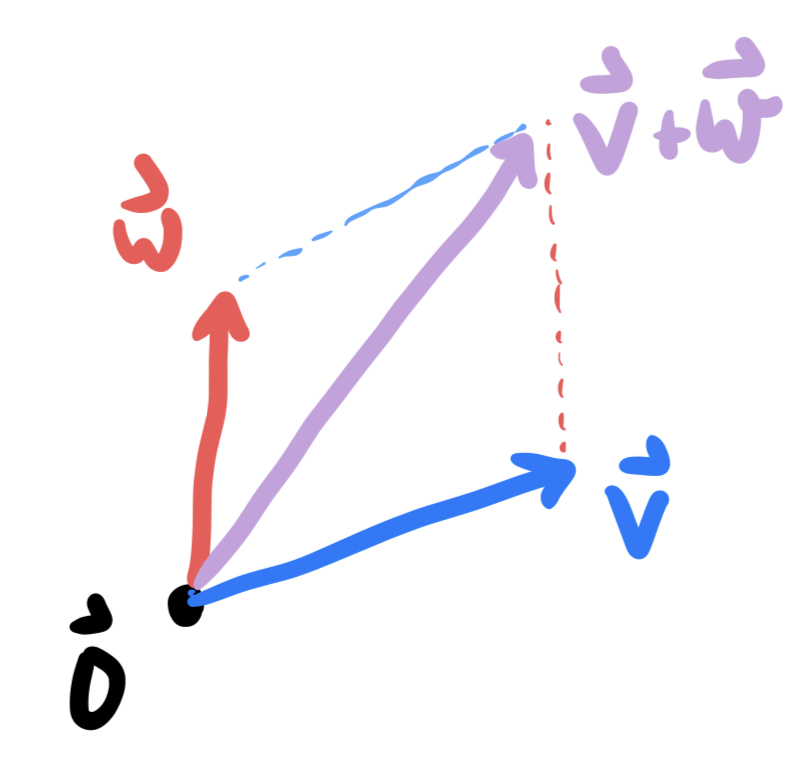
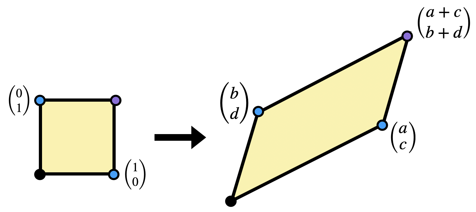
Definition 7.2 (Vector Addition) If \(u,v\) are two vectors, then their sum is the vector whose tip lies at the opposite side of the parallelogram spanned by \(u\) and \(v\). In coordinates, this is just the component-wise sum of the two vectors: \[u=\langle a,b\rangle\hspace{1cm}v=\langle c,d\rangle\] \[u+v=\pmat{a\\ b}+\pmat{ c\\ d}=\pmat{ a+c\\ b+d}\]
We will often see vector addition as a means of performing a translation: adding a vector \(\vec{v}\) shifts a point \(\vec{p}\) in the plane to a new point \(\vec{p}+\vec{v}\). Doing this simultaneously to all points in the plane slides the entire plane by the vector \(\vec{v}\). For example, if \(v=\langle 1,2\rangle\) then translation by v$ is the function \[(x,y)\mapsto \pmat{x \\ y}+\pmat{1\\ 2}=\pmat{x+1\\ y+2}\]
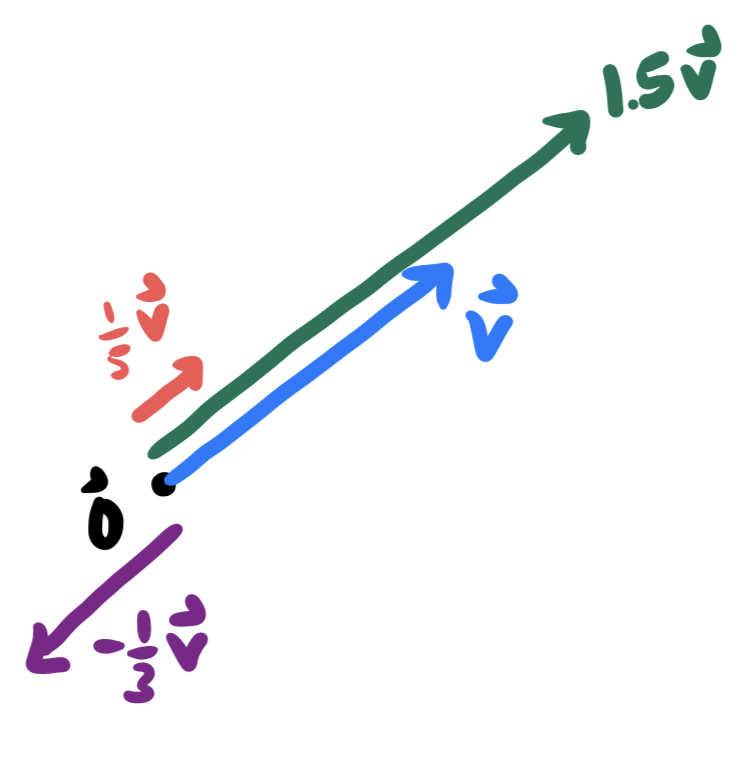
The second operation we can do to vectors is called scalar multiplication: this changes the length of a vector, without changing its direction (though, it flips the vector around backwards when the scalar is negative).
Definition 7.3 (Scalar Multiplication) If \(v\) is a vector and \(k\) is a number (scalar), we can create a new vector \(kv\) which points in the direction of \(v\), but is \(k\) times as long. In coordinates, if \(v=\langle a, b\rangle\) then \[kv=k\pmat{a\\ b}=\pmat{ka \\ kb}\]
The collection of all scalar multiples of a nonzero vector \(\vec{v}\) trace out the line through the origin, containing the vector \(\vec{v}\). Combining this with vector addition to allow for translations, we can easily describe lines in space in the language of linear algebra.

Definition 7.4 (Affine Lines) An affine line in a vector space is a function of the form \[\vec{\ell}(t)=\vec{p}+t\vec{v}\]
We can refer to such a line as the line through \(\vec{p}\) in direction \(\vec{v}\).
The Youtuber 3Blue1Brown has put together an excellent video series called the “Essence of Linear Algebra”. While much if it is beyond what we need for this course - I highly recommend watching the entire series! I’ll post throughout this article a few of the installments that are particularly relevant: here’s the introductory video on vectors.
7.2 Linear Maps
The operations of addition and scalar multiplication are of fundamental importance to vectors. Because of this, functions which play nicely with addition and scalar multiplication will
Definition 7.5 (Linear Maps) A function \(F\) between vector spaces is a linear map if:
- It preserves addition: \(F(u+v)=F(u)+F(v)\) for all vectors \(u,v\).
- It preserves scalar multiplication: \(F(cv)=cF(v)\) for all scalars \(c\) and all vectors \(v\).
It’s easy to find examples of functions which are not linear: all they have to do is violate one of these two properties. For example, \(f(x)=x^2\) is not linear since \(f(x+y)=(x+y)^2=x^2+y^2+2xy\) and \(f(x)+f(y)=x^2+y^2\), so \(f(x+y)\neq f(x)+f(y)\). In fact, most functions are nonlinear.
Example 7.1 (1 Dimensional Linear Map) The single variable function \(f(x)=2x\) is a linear map. To see this, we check both addition and scalar multiplication: \[f(x+y)=2(x+y)=2x+2y=f(x)+f(y)\] \[f(cx)=2cx=c2x=cf(x)\]
Of course, nothing about the 2 above is special the functions \(f(x)=mx\) - which we know from algebra classes to describe lines through the origin - are all examples of linear maps. Examples get more interesting in two dimensions:
Example 7.2 (2 Dimensional Linear Map) The function \(F(x,y)=(2x,x+y)\) is a linear map. Again, we just need to check addition and scalar multiplication. Let \(u=\langle u_1,u_2\rangle\), \(v=\langle v_1,v_2\), and \(c\) be any constant. Then check, using the rules we learned above, that \[F(u+v)=F(u)+F(v)\] \[F(cu)=cF(u)\]
Below is one relatively straightforward warm-up proposition using the definition of linearity, which nonetheless proves very useful: linear transformations send lines to lines.
Proposition 7.1 (Linear Maps Preserve Lines) If \(\ell(t)=p+tv\) is an affine line and \(F\) is a linear map, then \(F(\ell(t))\) is also an affine line.
Proof. This is just a computation, together with the definition of linear map and affine line. Plugging in \(\ell(t)\), we use that \(F\) preserves addition, so\(F(p+tv)=F(p)+F(tv)\). Next we use that \(F\) preserves scalar multiplcation, so \(F(tv)=tF(v)\). Putting it all together, \[F(p+tv)=F(p)+tF(v)\] Since \(F(p)\) and \(F(v)\) are constant vectors, this result is of the form \[\mathrm{vector}+t\cdot \mathrm{vector}\] which is the same form we started with: so its also an affine line.

Here’s 3Blue1Brown’s video on Linear Transformations and Matrices: it does an absolutely excellent job of displaying the geometric meaning of linear maps we just discovered above, as well as motivating the definition of matrices (which we define below).
7.3 Matrices
Linear maps are very constrained objects: the fact that they preserve addition and scalar multiplication tells us that its possible to reconstruct exactly what they do to any point whatsoever from very little data. We will mostly be concerned with linear maps from \(\RR^2\to\RR^2\), so I’ll use this as an example.
Say we know that \(L\) is a linear map, and we also know what happens when we plug in the vectors \((1,0)\) and \((0,1)\).
\[L(1,0)=(2,3)\hspace{1cm} L(0,1)=(-1,1)\]
How can we figure out what happens to \((x,y)\) after applying \(L\)? Well, first we use addition and scalar multiplication to break down the vector \((x,y)\) into simpler pieces.
\[(x,y)=(x,0)+(0,y)=x(1,0)+y(0,1)\] Then we can feed this linear combination into the function \(L\), and use the fact that it preserves these operations to our advantage:
\[\begin{align*} L(x,y)&=L(x(1,0)+y(0,1))\\ &= L(x(1,0))+L(y(0,1))\\ &= xL(1,0)+y L(0,1)\\ &= x(2,3)+y(-1,1) \end{align*}\]
We can further simplify this answer by using addition and scalar multiplication (again!):
\[\begin{align*} x(2,3)+y(-1,1)&= (2x,3x)+(-y,y)\\ &= (2x-y,3x+y) \end{align*}\]
Thus, from knowing only what \(L\) does to the vectors \((1,0)\) and \((0,1)\), we can deduce the entire formula for \(L\)
\[L(x,y)=(2x-y,3x+y)\]
The takeaway from this computation is that remembering what a linear map does to the standard basis vectors is of fundamental importance. In fact, this is exactly what the notation of a matrix is all about!
Definition 7.6 (Matrix) A matrix is an array of numbers. The following are all examples of matrices \[\pmat{1 &2}\hspace{0.5cm}\pmat{3\\ 7}\hspace{0.5cm}\pmat{1&2\\ 3&4}\hspace{0.5cm}\pmat{1&2\\ 3&4\\ 5&6}\]
Definition 7.7 (Matrix of a Linear Map) If \(L\) is a linear map, the matrix for \(L\) has its first column equal to the image of the first basis vector, the second column equal to the image of the second basis vector etc. In symbols, for a map from \(\RR^2\):
\[\pmat{| &| \\ L(1,0)&L(0,1)\\ | &|}\]
Example 7.3 (Matrix of a Linear Map) Consider the linear transformation \(L(x,y)=(2x-y,x+y)\). To find the matrix representation of \(L\), we just need to compute \(L\) on the basis vectors \((1,0)\) and \((0,1)\): \[L(1,0)=\pmat{2\\1}\hspace{1cm}L(0,1)=\pmat{-1\\1}\] The first of these is the first column of the matrix, and the second is the second column: that’s all there is to it! \[L=\pmat{2 & -1\\ 1&1}\]
Exercise 7.1 (Matrix of a Linear Map) Find a matrix for the following linear maps:
- \(L:\RR^2\to\RR^2\) which has the equation $\(L(x,y)=(4x-3y,2x+2y)\)
- \(M:\RR^2\to \RR\) which has the equation \(L(x,y)=2x-6y\).
- \(N\colon\RR^2\to\RR^3\) with \(L(x,y)=(x-y,x+z,y-z)\).
One of the best ways to understand linear maps is to visualize by hand how the transform the plane. Below is a picture drawn on the Euclidean plane.

Applying the linear transformation with matrix \(\smat{ 2&0 \\ 0 & 1}\) to this image turns the unit square of rectangles with sides \(\langle 2,0\rangle\) and \(\langle 0,1\rangle\). This transforms our image as below
Similarly, the transformation \(\smat{ -1/2&0 \\ 0 & 1}\) reflects the \(x\) axis, while leaving the \(y\) direction unchanged.

But all sorts of changes can happen! Linear maps can rotate, stretch, and squish our original square / image into any sort of parallelogram!
Exercise 7.2 Choose your own image on the plane (hand-drawn is great!), and draw a reference image of it undistorted, inside the unit square. Then draw its image under each of the following linear transformations:
\[\pmat{2&0\\ 0&2}\hspace{1cm} \pmat{1&1\\ 0&1}\hspace{1cm} \pmat{2&1\\ 1&1}\hspace{1cm} \pmat{0&-1\\1 &0}\]
7.3.1 Composition & Multiplication
Now we have at our disposal an easy-to-remember, easy-to-write notation for linear maps. All we do is store the results of the map on the standard basis! But how do we use this? How can we actually apply this linear maps to points? Looking back to our explicit example where \(\smat{2 & -1\\ 1&1}\) corresponds to \(L(x,y)=(2x-y,x+y)\), its clear: the first row stores the \(x\) and \(y\) coefficients of the first component, and the second row the coefficients of the second component.
Definition 7.8 (Applying a Matrix to a Vector) Given the matrix \(L=\smat{a&b\\ c&d}\), the linear transformation associated to this is \[L(x,y)=\pmat{a&b \\ c&d}\pmat{x\\ y}=\pmat{ax+b y\\ cx+dy}\] This formula is called the multiplication of a matrix by a vector.
Now we know how to apply a linear transformation, but how do we compose them? If I have two linear transformations, which are each a function \(\RR^2\to\RR^2\), I can do one after the other and get a new linear transformation. Abstractly, this is no problem. But if I actually want to compute things? Each linear transformation is represented by a matrix, how do I combine together two matrices in the right way to make a matrix for the result?
Example 7.4 Its perhaps most instructive to do this directly yourself. Start with two linear transformations, say \(L(x,y)=(x-y,2x+y)\) and \(M(x,y)=(3x+y,2x-5y)\), and compose them, simplifying the result as much as you can. What are the matrices for the three transformations \(L, M\) and \(M\circ L\)?
If you keep track of what you are doing during your simplification process, you’ll notice a pattern: you can deduce the matrix for the composition directly from the matrices of the transformations themselves!
Definition 7.9 (Matrix Multiplication) If \(L\) and \(M\) are linear transformations with the following two matrix representations \[L=\pmat{a&b\\ c&d}\hspace{1cm}M=\pmat{e&f\\ g&h}\] Then the linear transformation \(L\circ M\) has the following matrix:
\[L\circ M=\pmat{a&b\\ c&d}\pmat{e&f\\ g&h}=\pmat{ae+bg & af+bh\\ ce+dg & cf+dh}\]
The \(ij\)-entry of this matrix are formed by multiplying the \(i^{th}\) row of the first by the \(j^{th}\) column of the second element-wise, and adding up the results.
Early on in the course we will not have too much use for composing linear transformations explicitly, but once we reach the chapter on hyperbolic geometry - we will find this operation extremely useful to help explore spaces we struggle to visualize.
7.3.2 Inversion
How can we undo the behavior of a linear map?
Exercise 7.3 Given linear transformation \(L(x,y)=(x+y,x-2y)\), what vector does \(L\) send to \(\langle 3,4\rangle\)?
In the exercise above, we attempted to undo the behavior of \(L\) for a single vector. If we tried to do this for all vectors we would have a function that undoes the action of \(L\). We call this an inverse function
Definition 7.10 (Inverses) If \(L\colon X\to Y\) is a function, an inverse to \(L\) is a function \(M\colon Y\to X\) which undoes the behavior of \(L\). That is, for every \(x\in X\), if we apply \(L\) to get \(y=L(x)\in Y\), the inverse \(M\) takes \(y\) back to \(x\). Similarly if we start with \(M\) and then apply \(L\) they undo each other, so nothing changes. In symbols
\[M(L(x))=x\,\forall x\in X\hspace{1cm}L(M(y))=y\,\forall y\in Y\]
Exercise 7.4 Try to invert the linear map from above: \(L(x,y)=(x+y,x-2y)\). Find a function \(M(x,y)=(p x+qy,rx+sy)\) such that \(M(L(x,y))=(x,y)\) and vice versea.
If you do the above exercise carefully, you’ll find that the fact that the original linear map was \((x,y)\mapsto (x+y,x-2y)\) did not matter: you could have used any constants at all, and ran the same sort of argument for any linear transformation \((x,y)\mapsto (ax+by,cx+dy)\) at all! We will never have need to invert anything besides a \(2\times 2\) matrix, so the important takeaway from this section is the following general formula.
Proposition 7.2 (Inverse of a \(2\times 2\)) If \(L=\smat{a&b\\ c&d}\) is a linear transformation, it is invertible if \(ad-bc\neq 0\), and the inverse has matrix \[L^{-1}=\frac{1}{ad-bc}\pmat{d&-b\\ -c &a}\]
7.4 Determinants
In the formula for inverting a linear transformation above, a strange looking linear factor showed up in front of the matrix: the reciprocal of \(ad-bc\). What does this quantity measure?
A linear transformation \(L\) of the plane takes a square (spanned by the unit basis vectors \(e_1,e_2\)) to a parallelogram (spanned by the images of the basis vectors \(L(e_1)\) and \(L(e_2)\)). So, ratio by which \(L\) scales areas in the plane is captured by the area of the parallelogram spanned by \(L(e_1)\) and \(L(e_2)\). How can we find this area? It helps to draw a picture of the parallelogram we want. If \(L=\smat{a & b\\ c&d}\), then \(L\) sends the first basis vector to \(\langle a,c\rangle\) and the second to \(\langle b,d\rangle\):
We can actually find this area in a pretty satisfying way using just what we’ve proven about Euclidean geometry so far. We know the areas of squares, rectangles, and right triangles, so let’s try to write the area we are after as a difference of things we know:
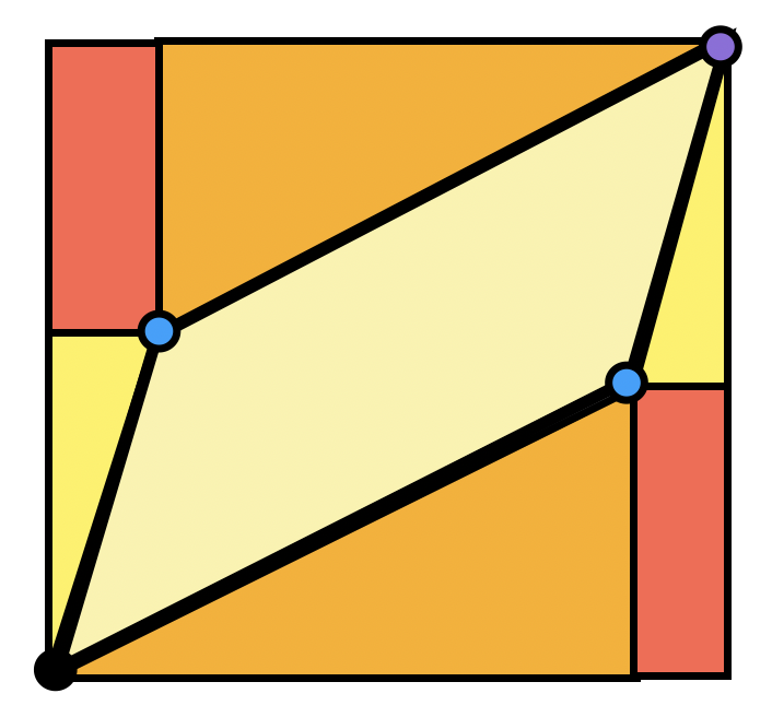
Exercise 7.5 Show the area of the parallelogram spanned by \(\langle a,c\rangle\) and \(\langle b,d\rangle\) is \(ad-bc\), using the Euclidean geometry we have done, and the diagram above.
Definition 7.11 (Determinant) The determinant of a linear transformation \(M=\left(\begin{smallmatrix}a&b\\c&d\end{smallmatrix}\right)\) is
\[\det M = \left|\begin{matrix}a &b\\c&d\end{matrix}\right| = ad-bc\]
Thus, the quantity we saw in the definition of the \(2\times 2\) matrix inverse was just \(1/\det\). This makes sense: if \(L\) scales up the area by a certain factor, then its inverse must undo that scaling, it must scale by the reciprocal!
Theorem 7.1 (Invertibility & The Determinant) A linear transformation is invertible if and only if its determinant is nonzero.
This theorem lets us think of the determinant as a tool to detect invertibility. If the determinant is zero, then the linear transformation takes a square to something of zero area: a point, or a line segment! And then information has been lost - the square has been crushed onto a smaller dimensional space - and there’s no undoing that.
So far we’ve figured out the meaning of the determinant when it is a positive number. But it can also be negative: what does it mean to scale area by a negative number? It’s easiest to see via an example - the matrix \(\smat{-1& 0\\0&1}\) has determinant \(-1\), and it flips an image upside down across the \(x\)-axis. This is the meaning of a negative determinant - a reflection!

We often refer to this concept formally with the term orientation. We say a function is orientation preserving if it does not reflect, or flip an image, and orientation reversing if it does. Thus, the determinant is not only an invertibility detector, but an orientation detector as well.
Definition 7.12 (Orientation Preserving) A linear transformation is orientation preserving if its determinant is a positive number.