12 Lines
Laying down the foundations at a deeper level than the Greeks, we have some work to do before we can hope to recover the axioms of Euclid. Indeed - no where in our foundations does the term line even appear: we are in the awkward position of being able to work with any curve we like, but we do not know which among them is a straight line!
To find the lines among the sea of curves, we need a good and precise definition. Definitions single out an important property characterizing the object being defined, and for that definition to be good, we would like that condition to be checkable within the framework we are building. So - Euclid’s definition of a line as a breadthless length is not going to do much for us here.
However, looking to history, we find several good candidate definitions among the properties of lines the ancients took as essential.
Definition 12.1 (Essential Properties of Lines)
Archimedes used as an axiom of length that the line segment between two points is the shortest among all curves connecting them. This could be turned upside down and directly used as the defining feature of lines: whichever curve is shortest, we call a line.
As a followup to the infamously unhelpful breadthless length Euclid states the important feature of a line being that the points lie evenly with themselves. This also requires a bit of translation, but if we can define what it means for a curve to turn, we could then specify straight lines as curves that do not turn.
The term line also shows up in phrases such as line of symmetry - for instance in discussing that the human form is left-right-symmetric. The fact that reflections fix a line is foundational to geometric arts like Origami, which is what allows the use of Euclidean geometry to describe the collection of creases made: they arise as lines of symmetry, so they are the lines of Euclid!
In fact all three of these things can be made into precise statements in our new geometry, and we can compute exactly what sort of curves satisfy each of them. The main purpose of this section is to do so, and to show that all three of them end up specifying exactly the same class of curves! This is one reason that lines are so important to geometry: they are the single objects sharing all three of these very natural properties!
12.1 Shortest
We start first with the insight of archimedes, and attempt to make precise the notion of shortest curve between two points. In doing so, we will actually first define line segment, and then use this to define lines more generally.
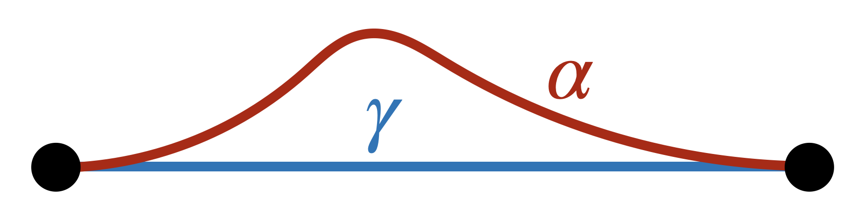
Definition 12.2 (Line Segment) Given two points \(p,q\in\EE^2\), a curve \(\gamma\) starting at \(p\) and ending at \(q\) is called a line segment if it is distance minimizing. That is, for all other curves \(\alpha\) from \(p\) to \(q\), we have \[\len(\gamma)\leq \len(\alpha)\]

This definition seems very powerful: if you know something is a line segment you know a lot about it: you know how its length relates to the length of every single other curve!
Theorem 12.1 (Segments of \(x\)-axis are Minimizers) Finite segments of the \(x\) axis, that is, curves of the form \[\gamma(t)=(t,0)\hspace{0.5cm}a\leq t\leq b\] are length minimizers.
Proof. First, we compute the length of the \(x\)-axis between \(0\) and \(L\) by integrating the infinitesimal lengths of \(\gamma\):
\[\gamma(t)=(t,0)\implies\gamma^\prime(t)=(1,0)\implies \|\gamma^\prime(t)\|=1\]
\[\len(\gamma)=\int_0^L\|\gamma^\prime(t)\|dt=\int_0^L dt=L\]
This of course is unsurprising! But its good to know explicitly that we have found a curve of length exactly \(L\). Now, let \(\alpha(t)=(x(t),y(t))\) be any arbitrary (regular)curve connecting \((0,0)\) to \((L,0)\).
Our goal is now to show that \(\len(\alpha)\geq L\), as this would mean no curve can have a length less than \(L\), and our segment of the \(x\)-axis above is indeed the shortest curve! The difficulty in doing so is that we know very little about \(\alpha\), and hence very little about its coordinate functions \(x(t),y(t)\). If \(\alpha\) is defined on the interval \([a,b]\) knowing that it starts and ends at \((0,0)\) and \((L,0)\) implies
\[\begin{matrix} x(a)=0 & x(b)=L\\ y(a)=0 & y(b)=0\end{matrix}\]
but this is essentially all we know. Nonetheless, let’s push onwards and see what we can learn about \(\length(\alpha)\) by writing out its definition.
\[\len(\alpha)=\int_a^b \|\alpha^\prime(t)\|dt=\int_a^b\sqrt{x^\prime(t)^2+y^\prime(t)^2}\,dt\]
Now we do some estimation: we know that whatever \(y\) is, \(y^\prime(t)^2\) is nonnegative - because its squared, after all! So \[y^\prime(t)^2\geq 0 \,\implies\, x^\prime(t)^2+y^\prime(t)^2\geq x^\prime(t)^2\]
We can then take the square root of both sides of this equation (which preserves inequalities) to get \[\sqrt{x^\prime(t)^2+y^\prime(t)^2}\geq \sqrt{x^\prime(t)^2}=|x^\prime(t)|\geq x^\prime(t)\]
Igoring all the middle terms in this string of inequalities, (and recalling the left hand side is the norm of \(\alpha^\prime\)) we see that
\[\|\alpha^\prime(t)\|\geq x^\prime(t)\hspace{0.5cm}\textrm{for all $t$}\]
Thus, as functions of \(t\), we see that the curve \(x^\prime\) lies below the curve \(\|\alpha^\prime\|\): since the area under the lower curve must be less than or equal to the upper, this inequality is still preserved after we integrate.
\[\int_a^b\|\alpha^\prime(t)\|\,dt\geq \int_a^b x^\prime(t)\,dt\]
But now we have really made some progress: on the right side here we are integrating a derivative, so we can use the fundamental theorem of calculus! The antiderivative of \(x^\prime(t)\) is just \(x(t)\) of course, so we evaluate at the endpoints:
\[\int_a^b x^\prime(t)\,dt = x(t)\Bigg|_a^b=x(b)-x(a)=L-0=L\]
And with that, we’ve done it! The integral on the left side was precisely the length of \(\alpha\), so \[\len(\alpha)\geq L\]
Now that we have a firm understanding of segments, how can we properly bootstrap this idea to a definition of lines? A line itself has no endpoints, and so is not a distance minimizing curve! However, it has the property that if you cut out any segment from it, that segment is distance minimizing. To say this formally, we need a word for “cut out a segment of a curve”
Definition 12.3 (Finite Segment of a Curve) Given a curve \(\gamma\colon\RR\to \EE^2\), a finite segment of \(\gamma\) is the restriction of \(\gamma\) to some finite interval \([a,b]\subset\RR\).

This makes the definition for a line completely precise:
Definition 12.4 (Line) A curve \(\gamma\) is a line if all of its finite segments are line segments.
This sounds pretty useless until we unpack it: since line segments are distance minimizers, this is saying that to be a line, a curve must have the property that it is distance minimizing between any two points it passes through! A strong condition indeed.
However, given the work we did above on segments of the \(x\) axis, we can now immediately apply this to the entire axis itself.
Corollary 12.1 (The \(x\)-axis is a line) Every finite segment of the \(x\)-axis is a distance minimizing line segment, so the \(x\)-axis is a line.
Well, after all this theory we have finally managed to track down one line in the plane! How can we find more? One option of course is to mimic the argument given here: with trivial modifications we can similarly prove that the \(y\) axis is a line, and that curves of the form \(x=a\) or \(y=b\) are all lines as well. But it would take a little more work (in the form of a clever \(u\)-substitution) to apply this further: we took big advantage of the fact that one of the coordinate derivatives was zero in our proof!
Instead, we take this as our first opportunity to use one of the most powerful ideas in modern geometry: symmetry. We proved that isometries preserve the length of all curves, and this has an important consequence: isometries send lines to lines!
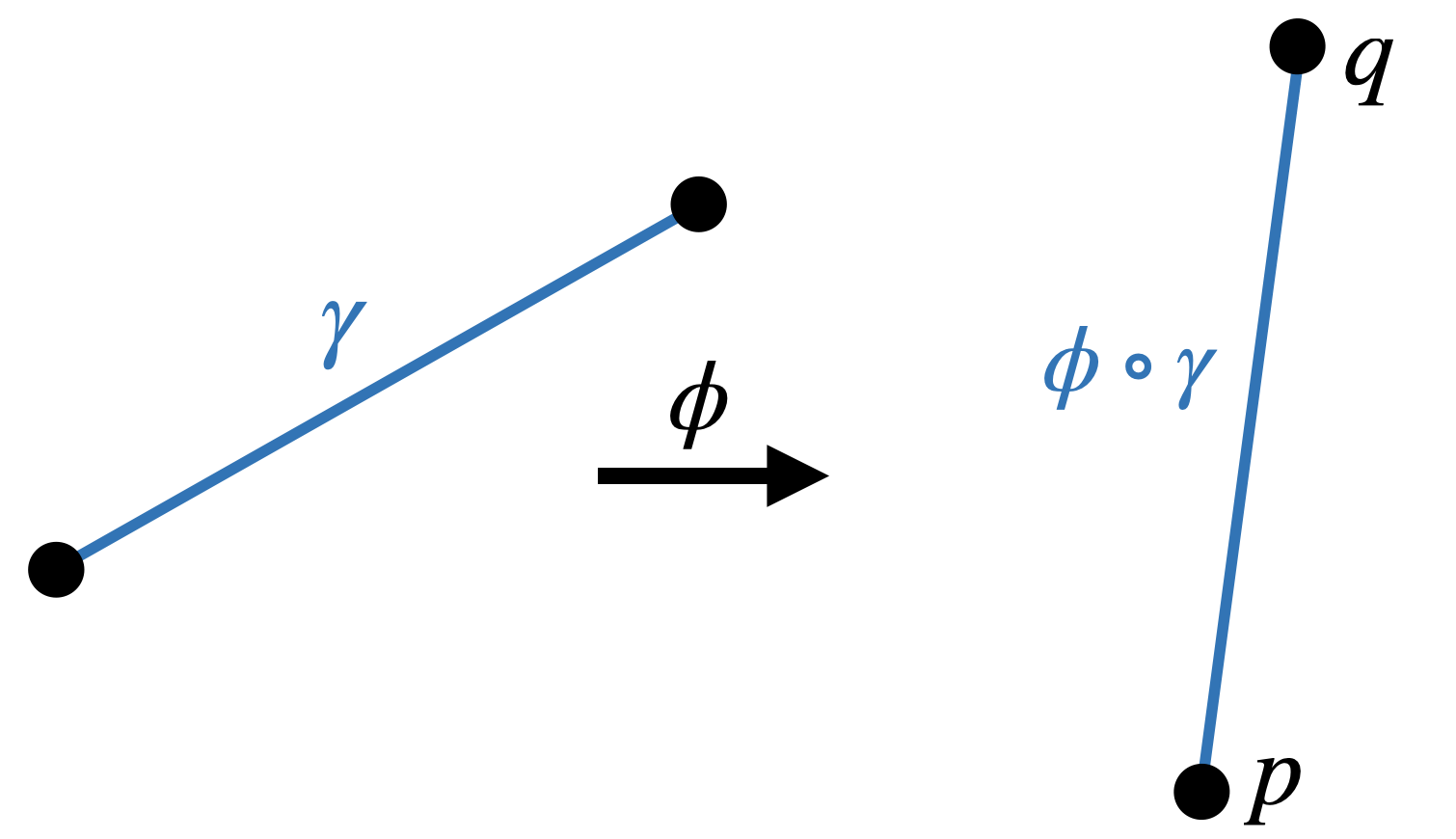
Theorem 12.2 (Isometries Send Lines to Lines) Let \(\gamma\colon\RR\to\EE^2\) be a line, and \(\phi\colon\EE^2\to\EE^2\) be an isometry. Then \(\phi\circ\gamma\) is also a line.
Proof. To argue that \(\phi\circ\gamma\) is a line, we need to show that all of its finite segments are length-minimizing. So, pick some arbitrary interval \([a,b]\subset\RR\) and look at the restriction of our curve to that segment, which goes from \(\phi(\gamma(a))=p\) to \(\phi(\gamma(b))=q\).
Assume for the sake of contradiction that this is not length minimizing: then there is some other curve \(\alpha\) connecting \(p\) to \(q\) which is of shorter length.

Now, apply the inverse function \(\phi^{-1}\) to everything: this takes the segment \(\phi\circ\gamma\) back to \(\gamma\), and takes \(\alpha\) to a new curve \(\phi^{-1}\circ\alpha\), starting and ending at the same points as the corresponding segment of \(\gamma\):

Since isometries preserve length, we know that since \(\alpha\) was shorter than \(\phi\circ\gamma\), we must now have that \(\phi^{-1}\circ\alpha\) is shorter than \(\gamma\)! But this is impossible: we assumed that \(\gamma\) itself was a line, so all of its segments are length-minimizing: there are no shorter curves!
Thus, its impossible that \(\alpha\) exists, so \(\phi\circ\gamma\) must have been the shortest segment between \(p\) and \(q\) after all. As all segments of this curve are distance minimizers, its a line!
This gives us an easy prescription to track down lines: we already know \(\gamma(t)=(t,0)\) is a line - and if we apply any isometry at all to this, we will get another line!
Corollary 12.2 (Affine Equations are Lines) Every linear equation \(f(t)=(at,bt)\) describes a line that passes through the origin. Every affine equation of the form \[\ell(t)=\pmat{at+c\\ bt+d}\] is also a Euclidean line.
Here we concentrate on the main case where \(\langle a,b\rangle\) is a unit vector. We comment below the proof on the small change needed when it is not.
Proof. Then, the rotation \(\phi=\smat{a&-b\\ b&a}\) taking \(\langle 1,0\rangle\in T_{(0,0)}\EE^2\) to \(\langle a,b\rangle\) is an isometry, so it sends lines to lines. Applying it to the \(x\)-axis \(\gamma(t)=(t,0)\), we see
\[\phi\circ\gamma(t)=\pmat{a& -b\\ b&a}\pmat{t\\0}=\pmat{at\\ bt}\]
Thus, \(t\mapsto (at,bt)\) is a line! Next, we can use the fact that for fixed \(c,d\) the translation \(\psi(x,y)=(x+c,y+d)\) is an isometry of \(\EE^2\), so
\[\psi(at,bt)=(at+c,bt+d)\] is also a line!
If \(v=\langle a,b\rangle\) is not a unit vector, then we can run the argument above using the unit vector \(\tfrac{v}{\|v\|}\). This gives us that the curve below is a line \[ \beta(t)= \left(\frac{a}{\sqrt{a^2+b^2}}t,\frac{b}{\sqrt{a^2+b^2}}t\right)\]
Since we know that the length of curves does not depend on their parameterization, we can speed up or slow down \(\beta\) by pre-composing it with another function, and not change the fact that it is distance minimizing! Speeding it up by \(t\mapsto \sqrt{a^2+b^2}t\) gives
\[\beta\left(\sqrt{a^2+b^2}t\right)=(at, bt)\] Thus \(t\mapsto (at,bt)\) is a line for any \(a,b\in\RR\)!
We saw in Theorem 12.2 that any isometry will carry a line to another line. The same is true more generally of similarities:
Exercise 12.1 (Similarities Send Lines to Lines) Let \(\gamma\colon\RR\to\EE^2\) be a line, and \(\sigma\colon\EE^2\to\EE^2\) be a similarity. Prove that \(\sigma\circ\gamma\) is also a line.
*Hint-replicate the proof of Theorem 12.2 as closely as possible, replacing the isometry \(\phi\) with the similarity \(\sigma\), and keeping track of the scaling factors of \(\sigma\) versus \(\sigma^{-1}\) (Proposition 11.4).
Using these tools, we can already start our process of rebuilding the Elements from below!
Theorem 12.3 (Proving Euclid’s Axiom I) Given any two points \(p,q\in\EE^2\), there is a line segment connecting \(p\) to \(q\).
Proof. Knowing that line segments are given by affine equations, we need just fine an affine equation \(\gamma(t)\) where \(\gamma(0)=p\) and \(\gamma(1)=q\). Perhaps the simplest such is \[\gamma(t)=p+(q-p)t\]
Theorem 12.4 (Proving Euclid’s Axiom II) Given a line segment between two points of \(\EE^2\), it can be extended indefinitely in either direction.
Proof. Let \(p,q\in\EE^2\) and define the line segment \(\gamma\colon [0,1]\to\EE^2\) by \(\gamma(t)=p+(q-p)t\) as in the previous theorem. To extend this line segment indefinitely, we need only extend the domain from \([0,1]\) to an arbitrary interval \([a,b]\) containing \([0,1]\).
The result is still an affine equation on a closed interval, and so still is a line segment by Corollary 12.2. And, as \([a,b]\) contains \([0,1]\) this new segment contains the original segment from \(p\) to \(q\), so it represents an extension of the segment.
12.1.1 Uniqueness of Lines
Above we proved the existence of lines, and found that all affine equations describe lines in the plane. But are these all the lines there are to be found? In fact they are - and we can confirm this with very little extra work: we had all the ideas in place already during the proof of Theorem 12.1.
Proposition 12.1 Segments of the \(x\)-axis are the unique distance minimizers between their endpoints.
Proof. Let \(\gamma(t)=(t,0)\) between \(t=a\) and \(t=b\), and \(\alpha(t)=(x(t),y(t))\) be a different curve with the same endpoints. Then since \(\alpha\) does not just trace the \(x\) axis, we must have \(y(t)\neq 0\) at some point. But \(y(a)=0\) and \(y(b)=0\) at the endpoints, so for \(y\) to go from zero to nonzero, it must have nonzero derivative on some interval.
But, this means that \(y^\prime(t)^2\) is strictly greater than zero on some interval, so \(\|\alpha^\prime(t)\|>\|\gamma^\prime(t)\|\), and \(\|\alpha^\prime(t)\|-\|\gamma^\prime(t)\|>0\) on some interval inside of \([a,b]\). Furthermore, since we already knew \(\|\alpha^\prime\|\geq\|\gamma^\prime\), this quantity is never negative. Thus
\[\int_a^b \|\alpha^\prime(t)\|-\|\gamma^\prime(t)\|\, dt >0\]
And, re-arranging the integral, this immediately implies \[\len(\alpha)=\int_a^b \|\alpha^\prime\|dt >\int_a^b\|\gamma^\prime\|dt=\len(\gamma)\]
Applying isometries to this, we can extend this result to any of the segments we already know:
Exercise 12.2 Prove that all Euclidean lines are given by affine equations. Hint: we already know that the affine equation \(\gamma(t)=(at+b,ct+d)\) defines a line. Can you show there is no curve of an equally short length, by using steps similar to the proofs Theorem 12.2 and ?cor-cor-affline-eqns-are-lines to reach a contradiction given that we just proved Proposition 12.1?
12.2 Straightest
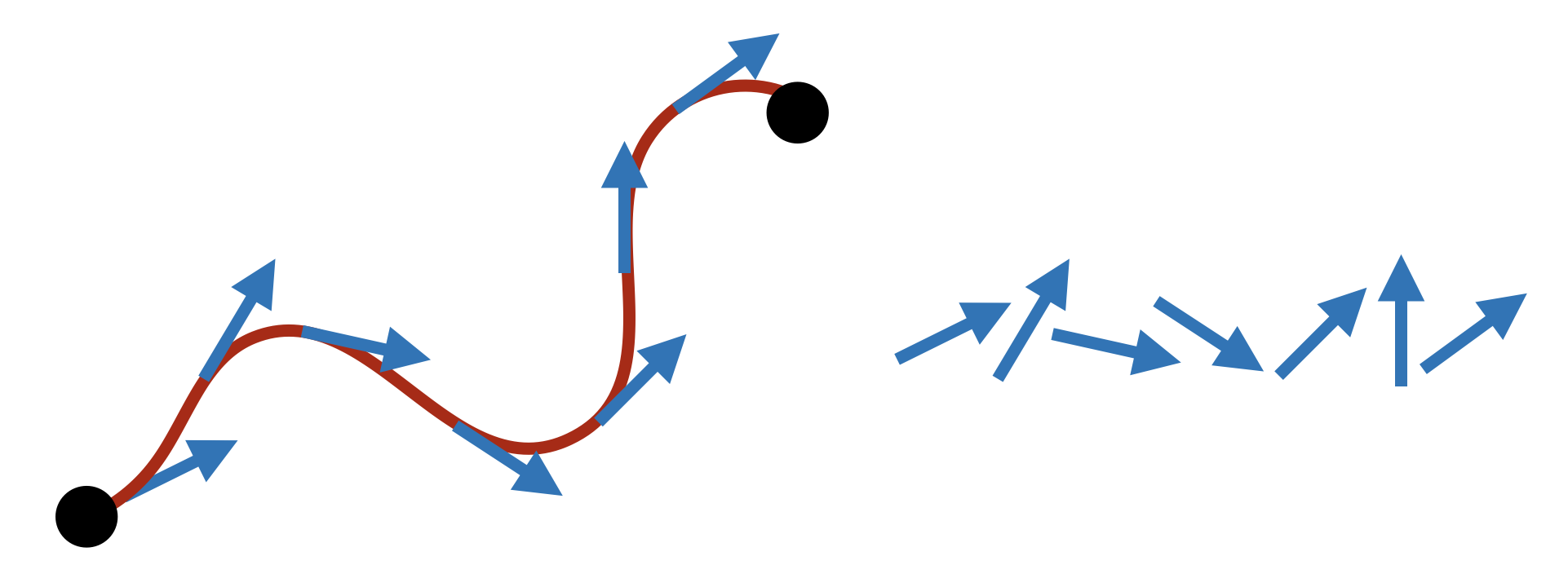
Another notion of line is “curve that doesn’t turn”. How do we make this precise? The unit tangent vector to a curve gives its direction, so we say a curve “turns” if the tangent changes direction.
The derivative of the tangent vector is acceleration, a “straight curve” would have acceleration zero.
Definition 12.5 (Straight) A curve \(\gamma\) is called straight if its tangent vector does not change. That is, if its acceleration is zero.
Remark 12.1. You might worry what it means to say that tangent vectors are constant, since each one of them technically lives in a different tangent space! This difficulty will be absolutely crucial to deal with later on, when space itself is curved. But here in \(\EE^2\), we can take advantage of the fact that we can make sense of the basis vectors \(\langle 1,0\rangle\) and \(\langle 0,1\rangle\) in each tangent space \(T_p\EE^2\): then constant just means that the components of the vectors are constant in time.
We’ve already done all of the hard work above, and we can now quickly confirm that this alternative definition picks out exactly the same class of curves.
Theorem 12.5 (Distance Minimizers are Straight) A curve \(\gamma\) is distance minimizing if and only if it is straight.
Proof. This is a direct computation, now that we’ve proven that every distance minimizer is given by a linear equation \(\ell(t)=p+tv\). Differentiating once leaves \(\ell^\prime(t)=v\), and differentiating twice gives \[\ell^{\prime\prime}(t)=\pmat{0\\0}\] Thus, \(\ell\) is straight.
To prove the other direction, we now assume we start with a straight curve \(\gamma\), and we wish to prove its distance minimizing. If \(\gamma\) is straight, then \(\gamma^{\prime\prime}=0\) and integrating twice we see that \[\gamma(t)=(at+c,bt+d)\] for some constants \(a,b,c,d\). Thus, \(\gamma\) is an affine curve, and we know affine curves are distance minimizers (Corollary 12.2). So, we are done!
This will turn out to be true in general: while we will have to be a little more careful when moving onwards to other geometries, curves that are straight will coincide with curves that minimize distance.
12.3 Folding
Finally we come to the third possible definition of line, and show that it also picks out the same collection of curves!
Definition 12.6 (Line of Symmetry) A fixed point of an isometry \(\phi\colon \EE^2\to\EE^2\) is a point \(p\) with \(\phi(p)=p\).
A curve \(\gamma\) is called a line of symmetry of \(\EE^2\) if there exists an isometry which fixes \(\gamma(t)\) for all \(t\).
This captures the intuitive notion of a crease from folding paper, or reflecting across a line: this swaps the two sides of the plane but leaves What are the fixed sets of reflections?
Proposition 12.2 (Reflecting in the \(x\)-Axis is an Isometry) The map \(\phi(x,y)=(x,-y)\) is an isometry of \(\EE^2\).
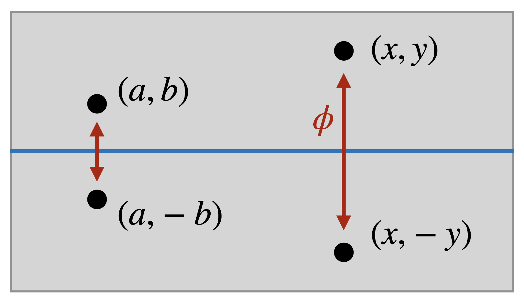
Proof. First, notice that \(\phi\) is actually a linear map, so we can write it as a matrix: \[\phi(x,y)=\pmat{1& 0 \\ 0& -1}\pmat{x\\ y}\]
Since \(\phi\) is linear, its derivative is constant and also equal to \(\phi\) at every point. Thus to check that it is an isometry, we only need to see that it does not change the length of any vectors.
Let \(v=\langle v_1,v_2\rangle_p\in T_p\EE^2\) be a tangent vector based at some arbitrary point \(p\). Then \[D\phi_p (v)=\pmat{1&0 \\ 0 &-1}\pmat{v_1\\ v_2}=\pmat{v_1\\ -v_2}\] And measuring lengths with the vector norm, \[\|D\phi_p(v)\|=\sqrt{v_1^2+(-v_2)^2}=\sqrt{v_1^2+v_2^2}=\|v\|\] Thus, \(\phi\) is an isometry.
This map fixes the line of points \((x,0)\) as it only negates the \(y\) component.Thus, the \(x\) axis is a line of symmetry! Similar to before, we can use isometries to prove that every affine curve is the fixed point of some reflection.
Exercise 12.3 (Reflections in Any Line) Prove that every affine curve is a line of symmetry. Hint: given an isometry that reflects in the \(x\) axis, can you build an isometry that reflects in any other line? Consider moving the line to the \(x\) axis, reflecting, and then moving back.
The converse is also true: that every line of symmetry is an affine equation: so this characterization of lines exactly agrees with the two previous. To prove this, we will need a bit better understanding of the isometries of Euclidean space, and so will postpone until that chapter,
12.4 Distance
So far in our development of Euclidean geometry, we have defined the length of a curve, but we have not defined any notion of distance between two points. This makes some sense, as the distance between two locations depends on how you get from one to the other, and that’s exactly what our definition captures!
However, now that we know there is a unique shortest curve between any two points, there’s a natural candidate for distance: the shortest possible path.
Definition 12.7 (Distance) The distance between two points \(p,q\in\EE^2\) is the length of the shortest possible curve starting at \(p\) and ending at \(q\).
Because of all of our hard work above, we can turn this rather abstract definition into something concrete and practical!
Theorem 12.6 (The Euclidean Distance) Let \(p\) and \(q\) be any two points in the plane. Then the Euclidean distance between them is given by
\[\dist(p,q)=\|p-q\|=\sqrt{(p_1-q_1)^2+(p_2-q_2)^2}\]

Proof. We can write down a distance minimizing curve from \(p\) to \(q\) as an affine equation: \[\gamma(t)=p+t(q-p)\] This is equal to \(p\) when \(t=0\) and \(q\) when \(t=1\). Thus, its length is given by the integral of \(\gamma^\prime\) over \([0,1]\). Computing the derivative is straightforward since \(\gamma\) is affine: \(\gamma^\prime(t)=q-p=(q_1-p_1,q_2-p_2)\), and so the length is
\[\begin{align*} \dist(p,q)&=\len(\gamma)\\ &=\int_{0}^1\|\gamma^\prime\|\, dt\\ &=\int_0^1\sqrt{(q_1-p_1)^2+(q_2-p_2)^2}\,dt\\ &=\sqrt{(q_1-p_1)^2+(q_2-p_2)^2}\int_0^1 dt\\ &=\sqrt{(q_1-p_1)^2+(q_2-p_2)^2} \end{align*}\]
Proposition 12.3 (Distance is preserved by isometries) If \(p\) and \(q\) are any two points in the plane and \(\phi\) is an isometry, then \[\dist(\phi(p),\phi(q))=\dist(p,q)\]

Proof. First, we start with the isometry case. Given two points \(p,q\) we can construct a line segment \(\gamma\) from \(p\) to \(q\) (Theorem 12.3), and as this segment is the minimizer we know its length accurately measures the distance: $\(\dist(p,q)=\len(\gamma)\).
Applying \(\phi\) we recall that isometries carry lines to lines (Theorem 12.2) to note that \(\phi\circ\gamma\) is a line segment between \(\phi(p)\) and \(\phi(q)\), and as line segments are distance minimizers, we know \[\dist(\phi(p),\phi(q))=\len(\phi\circ\gamma)\] Finally, we recall that isometries don’t change the length of curves (Theorem 11.2) to see \[\len(\gamma)=\len(\phi\circ\gamma)\] and stringing all these equalities together gives \[\dist(p,q)=\len(\gamma)=\len(\phi\circ\gamma)=\dist(\phi(p),\phi(q))\]
Exercise 12.4 If \(p\),\(q\) are any two points in the plane and \(\sigma\) is a similarity with scaling factor \(k\), prove \[\dist(\sigma(p),\sigma(q))=k\dist(p,q)\]
Hint: follow closely the argument for isometries above, replacing the theorems relating isometries, line segments, and lengths with the corresponding results for similarities.

It will often be useful to measure distances not just to points, but to more complicated objects in the plane.
Remark 12.2. We are avoiding a detail here, that anyone who has seen real analysis may be interested in. Sometimes, the minimum distance between \(p\) and a point in \(R\) doesn’t exist, but only the infimum of such distances does. However, we will never encounter such cases in this text.
Definition 12.8 (Distance to a Set) Let \(R\subset\EE^2\) be a region in the plane. Then the distance from a point \(p\in\EE^2\) to \(R\) is defined as the *shortest line segment connecting \(p\) to any point of \(R\), and is denoted \(\dist(p,R)\).

12.4.1 Useful Computations
'Now that we know exactly what lines are, we can convert elementary geometric problems - such as when they intersect - into algebraic problems, solvable via systems of equations. Here’s an example.
Exercise 12.5 (Intersecting Lines) Calculate the point of intersection between two lines \(ax+by=c\) and the the diagonal line \(x=y\). When is there no intersection?
With the ability to solve equations (since lines are given by affine equations, which are easy to work with!) we have developed a geometric superpower. To demonstrate this, we can use this to prove Playfair’s axiom (remember, this is equivalent to Euclid’s 5th Postulate!)
Proposition 12.4 Given any line \(L\) in \(\EE^2\), and any point \(p\in \EE^2\) not lying on \(L\), there exists a unique line \(\Lambda\) through \(p\) which does not intersect \(p\).
Exercise 12.6 Prove Proposition 1.
Hint: use isometries to help you out!
First, use an isometry to move \(L\) to the \(x\)-axis. Then, use another isometry to keep \(L\) on the \(x\) axis, but to move \(p\) to some point along the \(y\) axis (and possibly, use a reflection to then insure \(p\) has been moved to a point on the positive y axis, if you like!). Then, prove that through any point on the \(y\) axis there is a unique line that does not intersect the \(x\)-axis.
In addition to algebra, founding our new geometry on calculus makes all of these tools also available to us. As a first example, we will use our knowledge of derivatives to minimize the distance between a point and a line. Minimizing distance turns out to be a pretty common thing one needs to do in applications of geometry, and while straightforward theoretically (take the derivative, set it equal to zero), its annoying in practice because of the square root in the distance formula. But there is a nice trick to get around this:
Exercise 12.7 (Minimizing the Square: A Very Useful Trick!) Let \(f(x)\) be a differentiable positive function of one variable, and let \(s(x)=f(x)^2\) be its square. Show that the minima of \(s(x)\) and \(f(x)\) occur at the same points, by following the steps below:
First, assume \(x=a\) is the location of a minimum of \(f\). What does the first and second derivative test tell you about the values \(f^\prime(a)\) and \(f^{\prime\prime}(a)\)? Use this, together with the fact that \(f(a)>0\) to show that \(x=a\) is also the location of a minimum of \(s\) (using the second derivative test).
Conversely, assume \(x=a\) is the location of a minimum of \(s(x)\). Now, you know information about the derivatives \(s^\prime(a)\) and \(s^{\prime\prime}(a)\). Use this to conclude information about \(f^\prime(a)\) and \(f^{\prime\prime}(a)\) to show that \(a\) is a minimum for \(f\) as well.
This tells us anytime we want to minimize a positive function, we could always choose to find where its square is minimized instead, if that turns out to be easier. The main question is below, where without loss of generality we have taken the point to be the origin (as we could always slide it there via an isometry).
Exercise 12.8 (Closest Point on Line) Let \(L\) be the line traced by the affine curve \(\gamma(t)=\pmat{a t+ c\\ bt +d}\), and \(O\) be the origin, as usual. Calculate \(\dist(O,L)\)
Hint: use calculus to find the closest point on \(L\) to \(O\). Can you minimize the squared distance from \(\gamma(t)\) to \((0,0)\)?