25 Discovery
In this chapter we will embark on our final journey in the Foundations of Geometry, and construct the third flavor of geometry: hyperbolic space.
To do so, we will draw on all of our knowledge from the course, from the Greeks, through calculus, to spherical geometry and its expression in maps.
The discovery of hyperbolic geometry was one of the big mathematical achievements of the previous millennium, as not only did it open our minds to the much richer geometric world mathematicians now work in, but it also definitively answered the most important outstanding question of the Greeks. So, it is only fitting, that in this final chapter we look back to where we began.
25.1 Prelude: The Legacy of the Greeks
The ancient Greeks were right to feel proud of their progress in geometry: after a couple of centuries of deep thought they mastered the axiomatic method, and went forth to prove hundreds upon hundreds of theorems answering almost every question they had about the geometry of 2 and 3 dimensional space.
Almost.
The golden age of Greek mathematics closed with a few important open problems remaining, that they posed to the generations of the future. Three of these were questions about the specifics of greek method of constructing geometric figures using a ruler and compass:
- Doubling the cube: given a cube, use a ruler and compass to construct a new cube with double the volume.
- Squaring the Circle: Given a circle, use a ruler and compass to construct a square with the same area as the circle.
- Trisecting angles: Given an arbitrary angle, use a ruler and compass to draw two new lines which divide it evenly in thirds.
The deep knowledge of greek mathematicians becomes even more clear as we look back at these problems as guiding lights for mathematics over the last two thousand years. While today all have been solved, it took until the 1800’s, the answers required an entirely new branch of mathematics, and they were all answers the greeks and their successors never imagined:
- Doubling the cube with a ruler and compass is impossible.
- Squaring the circle with a ruler and compass is impossible.
- Trisecting an arbitrary angle with a ruler and compass is impossible.
Unfortunately: we will not answer these three in this course. It turns out the new idea needed to answer all three of these questions came from abstract algebra - specifically, from the theory of fields, and field extensions! So while the questions are pure geometry, their resolutions are arguments in algebra! If you are currently in abstract algebra - please feel free to come ask me about them!
We will instead focus our attention on the much larger problem the greeks left open: not a problem about some particular method of drawing geometric figures, but about the nature of geometry itself.
- Prove the fifth postulate from the remaining four (or show that this is impossible).
This question was worked on for approximately two thousand years by the greatest mathematical minds, with essentially no success until its eventual resolution 200 years ago (around 1823). It is one of the great joys of undergraduate mathematics to be able to seriously engage with the mathematics of the intervening two thousand years, and be able to fully understand the answers to these lasting questions, and this course has essentially been designed to exposit this problem’s solution. So, lets begin!
25.1.1 Disproof by Counterexample
Perhaps, like the other questions of antiquity, the reason the greeks failed to prove the fifth postulate from the other four is that this is also impossible. One way to show a claim is impossible is by finding a counterexample, and that is the approach that we will take here. But a counterexample to what? If the question is to “prove Postulate V from postulates I-IV”, then a counterexample would be a geometry which satisfies the first four axioms, but for which the fifth is false. The existence of such a geometry would spell doom to any hope of proving the fifth in the same way that the number 4 spells doom to any hope to proving that all numbers greater than 1 are prime. It would once and for all settle the question, and in the same style as the other greek resolutions: it seems that when it comes to geometry, the only things the greeks didn’t succeed at were impossible!
But while the dream of producing a counterexample is clear, the actual process for doing so is not. While its easy to write down a geometry in our modern definition (you just need to give me a set of points, and rules for doing calculus with infinitesimal arc lengths and angles at each point), most everything you will write down will not satisfy all four of the first axioms of the greeks.
The first and third axioms basically state that “space doesn’t have any holes, tears, rips or edges in it”: you can always connect two points with a line segment and once you have a line segment you can always sweep it around in a circle.
The second axioms says something about space being infinite: we already saw that this fails on finite spaces like the sphere. But its more particular than that - it can also fail on some infinite spaces like the cylinder, where geodesics can be extended indefinitely in one direction, but not in others. For axioms 2 to be satisfied in the way the Greeks originally stated it, space needs to be “infinite in all directions”.
A more modern reading of this axiom by Bernhard Riemann in the 1800s replaces it with a weaker statement that only says geodesics can’t come to an “edge” you have to be able to continue forwards forever, but its OK if you retrace your steps. This allows the sphere to be worked with more naturally in the context of axiomatic geometry.

The axiom that is hard to satisfy is the fourth: all right angles are equal. Remember that when making this precise, we realized it implies that space is both homogeneous and isotropic: you can move any point to any other, and you can rotate about any point, in any direction. This axiom is the key to a lot of what we do when proving things: we always move something to the origin, or to the north pole to simplify our calculations, and justify it by our proofs that the sphere and plane are homogeneous. But any little change whatsoever to the sphere or plane generally produces something that is not homogeneous:

Thus, its relatively easy to produce a geometry which satisfies axioms 1,2 and 3 but fails 4, and its also possible (but harder) to produce a geometry which satisfies 1,3, and 4, but fails 2 (the sphere). Unfortunately neither of these help us in our quest for a counterexample. Even though we proved on the sphere that the parallel postulate is false (we found a triangle with three 90 degree angles: so the angles on one side added up to 180 yet the lines still intersected!), this does nothing towards our goal, as it didn’t satisfy the other four to begin with!

To build our counterexample, we want to take as much inspiration from the sphere and the plane as possible - since these are the only two geometries that we know of that satisfy Postulate 4. But we want our new creation to be infinite like Euclidean space, and yet fail the parallel postulate like the sphere.
25.2 A Radical Idea
While we often speak as though we have studied two geometries so far - Euclidean and spherical - this actually isn’t quite right. Indeed, we proved along the way that there is actually a different sphere geometry for each radius! More precisely, we’ve studied the Euclidean plane, and a whole 1-parameter family of spherical geometries
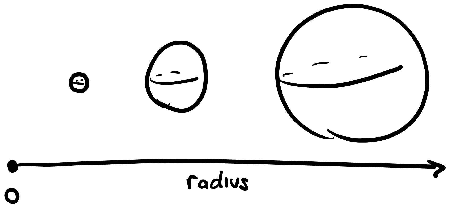
The sphere geometries are all closely related to one another, (by a similarity that is not an isometry) and so their geometric formulae are all closely related as well. This allowed us to start with careful study of the unit sphere and then expand our knowledge to spheres of any other radius: for example, deriving the formulas for circumference and area of circles on a sphere of radius \(R\):
\[C(r)=2\pi R\sin\left(\frac{r}{R}\right)\] \[A(r)=2\pi R\left(1-R\cos\left(\frac{r}{R}\right)\right)=4\pi R^2 \sin^2\left(\frac{r}{2R}\right)\]
Exercise 25.1 Derive this formula for the area of a circle on the sphere of radius \(R\): use the fact that you found the circumference on a previous homework, and that area is teh integral of circumference
\[A(r)=\int_0^r C(r)\,dr\]
Then apply a trigonometric identity to simplify things and get the second expression.
The same ideas apply to other important formulas in geometry like the spherical pythagorean theorem: you found this on the homework to be \(\cos(c)=\cos(a)\cos(b)\) on the unit sphere, which generalizes on the sphere of radius \(R\) to
\[\cos\left(\frac{c}{R}\right)=\cos\left(\frac{a}{R}\right)\cos\left(\frac{b}{R}\right)\]
And the area of a spherical triangle, which is \(A=\alpha+\beta+\gamma-\pi\) on the unit sphere, and
\[A = R^2(\alpha+\beta+\gamma-\pi)\]
on the sphere of radius \(R\). This continues for the spherical trigonometry of right triangles. Consider the triangle with angles \(\alpha,\beta\), opposite sides \(a,b\) and hypotenuse \(c\). On the unit sphere we had the relations \(\sin \alpha=\frac{\sin a}{\sin c}\) and \(\cos\alpha = \frac{\tan b}{\tan c}\). Thus, on the sphere of radius \(R\) we have
\[ \sin \alpha=\frac{\sin \frac aR}{\sin \frac cR} \hspace{1cm}\cos\alpha = \frac{\tan \frac bR}{\tan \frac cR}\]
Then rather separately, we had the geometry of the Euclidean plane, where we spent the first half of the semester carefully confirming all of the results we knew from earlier education:
\[C_{\EE^2}(r)=2\pi r\hspace{1cm}A_{\EE^2}(r)=2\pi r^2\] \[c^2=a^2+b^2\] \[\sin\alpha = \frac{a}{c}\hspace{1cm}\cos\alpha =\frac{b}{c}\]
These formulas are different than those of the sphere, but not wholly so. Indeed - we saw earlier a hint at the connection, by recovering the Euclidean pythagorean theorem from the spherical one, as the radius of the sphere goes to infinity. But this wasn’t an accident: if you take \(\lim_{R\to\infty}\) in any of the spherical formulas above, you’ll recover the Euclidean counterpart!
:::{#rem-euc-triang} Here of course there’s no analog of the formula giving a triangles area in terms of its angle sum, as in Euclidean space the angles do not determine the size of a triangle at all!:::
Exercise 25.2 (Circle Area and the Euclidean Limit:) Let \(C_R(r)=2\pi(1-R\cos(r/R))\) be the area of a circle of radius \(r\) on \(\SS^2_R\). Prove that as \(R\to\infty\) this converges to the Euclidean formula \[\lim_{R\to\infty}C_R(r)=\pi r^2\]
Exercise 25.3 (Trigonometry and the Euclidean Limit) Show that in the limit \(R\to\infty\), the trigonometric formulas for spherical right triangles converge to their Euclidean counterparts.
\[\lim_{R\to\infty}\frac{\sin \frac aR}{\sin \frac cR} =\frac{a}{c}\] \[\lim_{R\to\infty}\frac{\tan \frac bR}{\tan \frac cR} =\frac{b}{c}\]
This is even true for the maps we’ve studied! For example you’re calculating the scaling factor for stereographic projection on the homework, and finding the map-dot product on the plane:
\[(v\cdot w)_\map = \frac{4R^4}{(R^2+X^2+Y^2)^2}(v\cdot w)\]
Thus, this tells us how to rescale the Euclidean dot product \(v\cdot w\) depending on our location \((x,y)\in\EE^2\), so that the result accurately reflects teh true dot product on the sphere. But when \(R\to\infty\), this true dot product becomes the Euclidean plane!
Exercise 25.4 (Maps and the Euclidean Limit) Show that as \(R\to\infty\), the scaling factor of stereographic projection becomes a constant. Thus, the map now treats vectors based at different points all the same - just like Euclidean geometry! (In fact, the result is Euclidean geometry).
Because this all fits together so nicely, we might picture the geometries we have discovered so far as forming a line (the spheres) with teh Euclidean plane off at infinity.

This picture suggests a radical idea: as we increase the radius of the sphere, we keep our geometry nice and homogeneous but make it larger: getting closer to satisfying postulate 2. Once we go all the way to \(R=\infty\) we reach Euclidean space, where Postulate 2 is satisfied! What if we kept going? Can we go beyond Euclidean space, pushing the radius past \(\infty\), and uncover new spaces, where Postulate 2 is true, but - like the spheres - the parallel postulate is false?

25.2.1 To Infinity and Beyond
Theres one obvious problem with our grand plan however: what could it possibly mean to go beyond infinity? We can’t even go to infinity rigorously - everything must be done in terms of limits. We want to use the formulas we’ve worked hard to develop this semester as a guide for whatever new geometry lies on the other side, but the formuls are no good if the first step is “plug in a number larger than \(\infty\)” when in fact there are no such things.
What we need is a change in perspective. We would like to replace our discussion of \(\lim_{R\to \infty}\) with something we can evaluate at a finite number. And, curvature provides the key. When studying spherical geometry, we proved there was an inverse relationship between radius and curvature: the bigger a sphere the less it was curved, and the smaller the sphere the larger its curvature. More precisely we showed that
\[\kappa = \frac{1}{R^2}\]
Thus, we can go to any of our formulas above, and directly replace any occurrences of \(R^2\) with \(\kappa\) without changing any of the math. For example, the circumference \(C_R(r)=2\pi R \sin(r/R)\) becomes
\[C_\kappa(r)=\frac{2\pi}{\sqrt{\kappa}}\sin(\sqrt{\kappa}r)\]
where we’ve re-arranged the relationship of radius and curvature above to be able to substitute \(R=\frac{1}{\sqrt{\kappa}}\).
Exercise 25.5 Give the analogs of other spherical geometry formulas in terms of curvature.
The euclidean limit now is no longer \(R\to\infty\), but rather \(\kappa\to 0\): and it now makes perfect conceptual sense to ask what happens if we keep going? We should just get \(\kappa = 0\), and then - pushing onwards - get negative values of \(\kappa\)!

There’s just one problem with this: it doesn’t seem to work when we look at our formula. Indeed, when \(\kappa=0\) the circumference is an indeterminate form \(0/0\) (since \(\sin(0)=0\)), and when \(\kappa<0\) we are trying to plug a negative number into a square root. But this is not as serious of a problem as it seems at first. We’ve expressed this function in one way, using the function \(\sin\) which we invented for the study of circles in Euclidean geometry. But mathematics doesn’t care how we write things down in symbols - those are human inventions. And we can write the exact same function using a series expansion, since right after our definition of \(\sin\) we derived its series $\(\sin x = x-x^3/3!+x^5/5!-\cdots\)
\[C_\kappa(r)=\frac{2\pi}{\sqrt{\kappa}}\left(\sqrt{\kappa}r-\frac{1}{3!}(\sqrt{\kappa}r)^3+\frac{1}{5!}(\sqrt{\kappa}r)^5-\cdots\right)\] \[=\frac{2\pi}{\sqrt{\kappa}}\left(\sqrt{\kappa}r-\frac{1}{3!}\sqrt{\kappa}^3r^3+\frac{1}{5!}\sqrt{\kappa}^5r^5-\cdots\right)\]
We can simplify this by noting that every single term in the parentheses contains a \(\sqrt{\kappa}\), and so we can safely factor one out, cancelling its counterpart in the denominator of \(2\pi\): \[=2\pi \left(r-\frac{1}{3!}\kappa r^+\frac{1}{5!}\kappa^2r^5-\cdots\right)\]
This formula is exactly equal to the formula we started with, just expressed in another notation. BUt this other notation is much more suggestive when we are looking to be bold, and think about what happens if we explore beyond the original \(\kappa>0\) regime in which we derived it. Indeed - this formula is completely well-defined for all \(\kappa\)! So we may take \(\kappa\) zero, and we recover directly \(C_0(r)=2\pi r\) - Euclidean geometry!
What happens when \(\kappa\) is negative? Well, if we look at the formula, we see that each term is multiplied by an
Half of the terms (those with odd powers of \(\kappa\)) change sign! This makes ALL the signs positive!! Here we’ve written \(\kappa = -|\kappa|\) and used \(|\kappa|\) in the formula to cancel these signs and emphasize that everything is positive \[C_{\kappa}(r)=2\pi(r+\frac{1}{3!}|\kappa| r^3+\frac{1}{5!}|\kappa|^2 r^5+\cdots)\]
The case we will be most interested in is when we push \(\kappa\) all the way to negative 1. Here the circumference function is just
\[C(r)=2\pi(r+\frac{1}{3!}r^3+\frac{1}{5!}r^5+\cdots)\]
What is this new function like, qualitatively? In making all the terms the same sign, we prevent all the cancellation that happens in the series expansion for \(\sin\) and \(\cos\) that keeps them bounded in size. Instead, this function gets larger with each term we add, in the end growing faster than any polynomial! This means if there really is some space for which this is the circumference formula, circles here would be very very large. Since smaller-than-Euclidean circles signifies positive curvature, bigger-than-Euclidean circles hints that the space will have negative curvature. But we can do better than that! We have an exact, quantitative formula for curvature involving circle’s circumference, after all.
Exercise 25.6 Let \(k<0\). Prove that a space with the circumference function \[2\pi(r+\frac{1}{3!}|\kappa| r^3+\frac{1}{5!}|\kappa|^2 r^5+\cdots)\] has curvature \(\kappa\), by computing the limit
\[\lim_{r\to 0^+}\frac{3}{\pi}\frac{2\pi r-C(r)}{r^3}\]
This tells us that if we construct a space whose circumference-to-radius-function is as above, then this space necessarily has curvature \(\kappa\). Doing so will create for us a space of every possible value of negative curvature, just as varying the radius of a sphere produces a space of every possible positive curvature. Such spaces are called hyperbolic
Definition 25.1 (Hyperbolic Geometry) Given a negative number \(\kappa\), hyperbolic geometry of curvature \(\kappa\) is denoted \(\HH^2_\kappa\), and is the space where at every point, the circumference of circles grows as \(C_\kappa(r)\). When \(\kappa=-1\), we often shorten this to just hyperbolic geometry* and denote it by \(\HH^2\).
Remark 25.1. It’s reasonable to wonder if this uniquely defines a space: after all, all we have done is say how the circles (and thus, the curvature) behaves. This is a good thing to think about, and it was resolved in 1839 by Minding’s Theorem which states that if two spaces have the same constant curvature, then they are locally isometric to one another.
To learn about this new hyperbolic space, we will push this technique as far as we possibly can: starting with a formula on the sphere, and pushing it to its limit (infinite radius, zero curvature) and beyond to the realm of negative curvature. In doing this we’ll see the function we met above - like the sine but with all the terms positive, is actually just the tip of the iceberg. There is a whole collection of parallel universe trigonometry functions out there, defined analogously. And since these functions will play a large role in our further development, now is a good time to pause and get ourselves acquainted.
25.3 Interlude: Hyperbolic Functions
Definition 25.2 (Hyperbolic Sine and Cosine) The hyperbolic sine and cosine function are defined by their series expansions, which are identical to those for \(\sin\) and \(\cos\), except that the sign of all coefficients have been made positive:
\[\sinh(x)=x+\frac{x^3}{3!}+\frac{x^5}{5!}+\frac{x^7}{7!}\cdots\] \[\cosh(x)=1+\frac{x^2}{2!}+\frac{x^4}{4!}+\frac{x^6}{6!}\cdots\]
Remark 25.2. The function name \(\cosh\) is pronounced as it is spelled, but \(\sinh\) is pronounced sinch in the US and shine in the UK.
To begin to develop intuition for these functions, we should take a look at their graphs. The first major revelation is that unlike the usual trigonometric functions, neither are periodic!
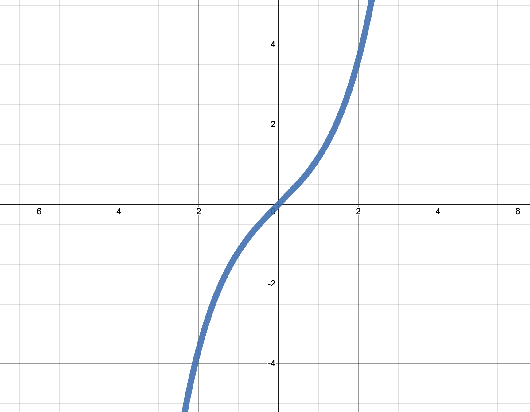

Also, they seem to grow extremely fast. How fast? We can actually quantify it by relating these functions to exponentials. Since \(\sinh\) contains all the odd terms of the series for \(e^x\) and \(\cosh\) contains all the even terms, we can see that \[\sinh(x)+\cosh(x)=e^x\]
Exercise 25.7 (Hyperbolic Functions in terms of Exponentials) Show that we can actually express the hyperbolic trigonometric functions in terms of exponentials:
\[\sinh(x)=\frac{e^x-e^{-x}}{2}\hspace{1cm}\cosh(x)=\frac{e^x+e^{-x}}{2}\]
Because \(e^{-x}\) quickly becomes small, this gives us a very precise understanding of just how quickly \(\sinh\) and \(\cosh\) grow. For \(x>>1\) we have
\[\cosh(x)\approx \sinh(x)\approx \frac{e^x}{2}\]
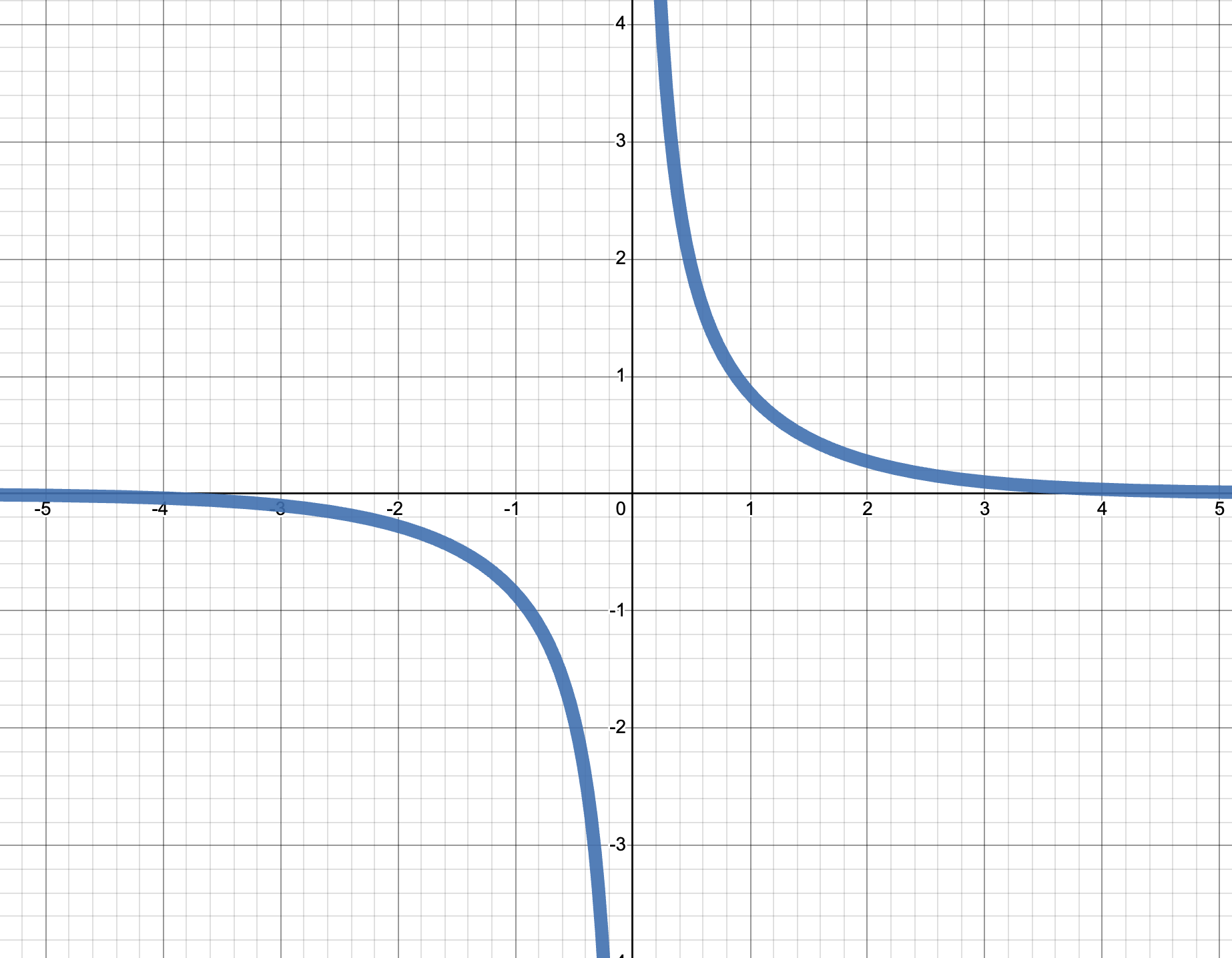
In direct analogy with regular trigonometry, starting from \(\sinh\) and \(\cosh\) we can build up a family of other hyperbolic trigonometric functions: (The first two of these are often pronounced tanch and coth. I am too scared to attempt to pronounce the second two)
Definition 25.3 (Other Hyperbolic Functions) \[\tanh x= s\frac{\sinh x}{\cosh x}\hspace{1cm}\coth x = \frac{\cosh x}{\sinh x}\] \[\operatorname{sech} x = \frac{1}{\cosh x}\hspace{1cm}\operatorname{cschs} x = \frac{1}{\sinh x}\]
Knowing what some of these look like as well will be important, so let’s take a minute to think about their graphs. How should \(\tanh\) behave? Well, both \(\sinh\) and \(\cosh\) are growing exponentially at the same rate, so their ratio should be approximately \(1\) for large inputs. And, \(\sinh\) is odd whereas \(\cosh\) is even, so the quotient is an odd function: passing through \(0\) with horizontal asymptotes at \(\pm 1\)!
Thus, \(\coth(x)=1/\tanh(x)\) should also asymptote to \(\pm 1\), but always be larger in absolute value, diverging to \(\pm\infty\) at the origin.
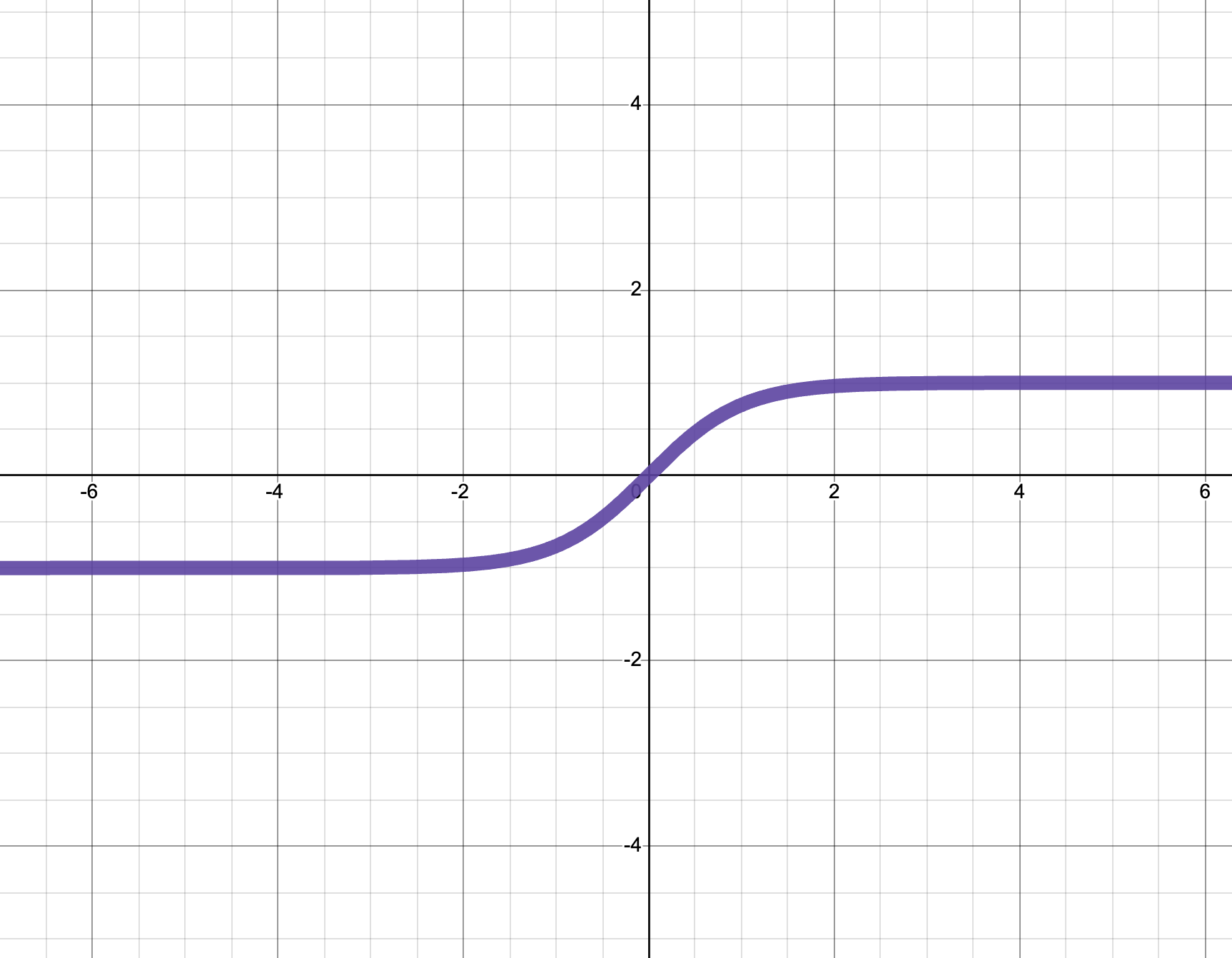
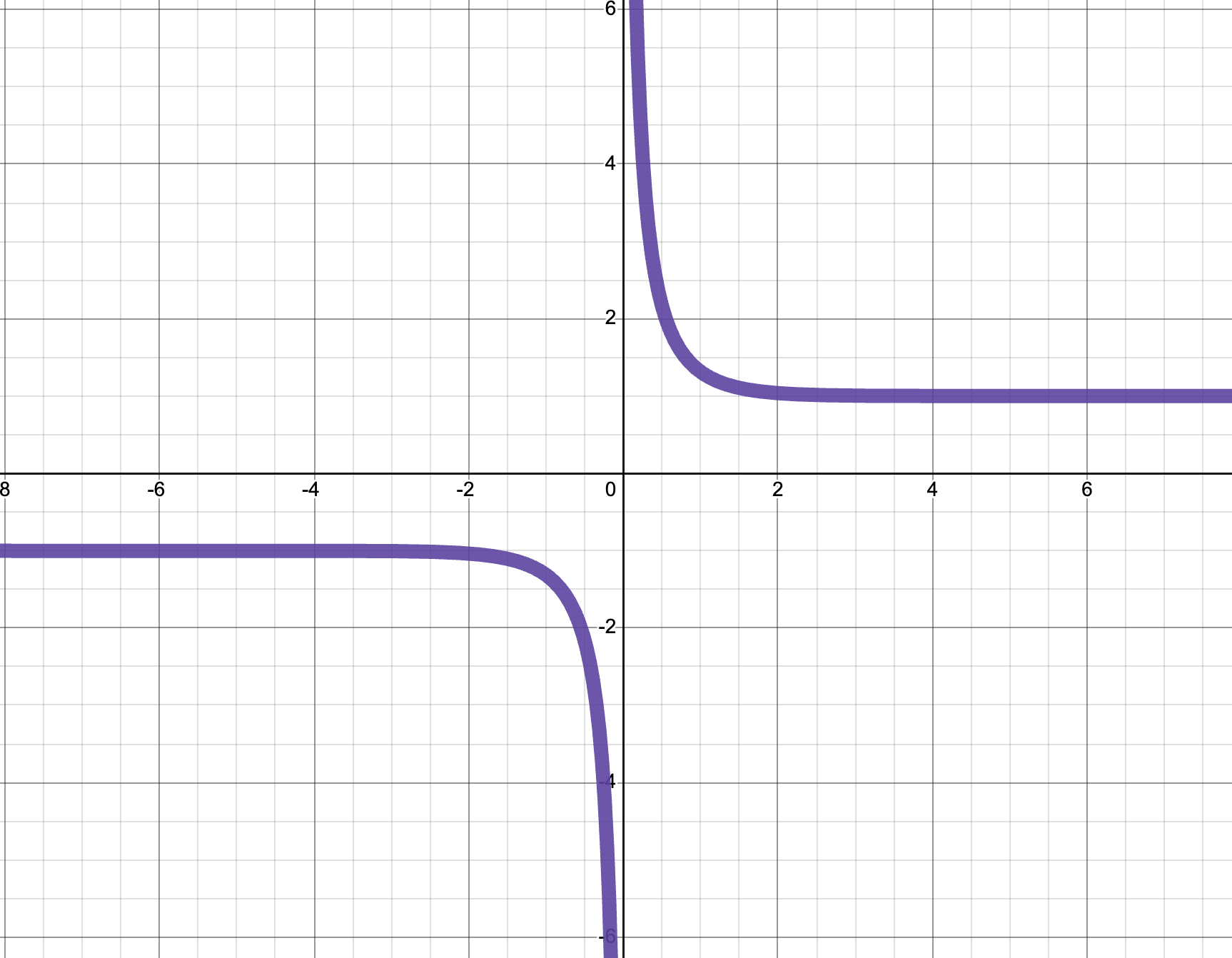
The reciprocals sech and csch of \(\cosh\) and \(\sinh\) share similar behavior, both asymptoting to \(0\), while the hyperbolic secant stays bounded in \([0,1]\) and the hyperbolic cosecant diverges at the origin.

These functions satisfy many analogous identities to the standard trigonometric ones as well, which can be proved directly from their definition:
Exercise 25.8 (Hyperbolic Trigonometric Identities) Prove that \[\cosh^2(x)-\sinh^2(x)=1\] Use this to deduce that \[\operatorname{sech}^2(x)+\tanh^2(x)=1\] These identities are the same as the Euclidean versions but with the sign switched! Hint: the formula relating to exponentials!
Exercise 25.9 Derive this trigonometric identity: \[\sinh(2x)=2\sinh(x)\cosh(x)\]
For the hyperbolic functions it turns out that calculus is even simpler than in the Euclidean case:
Exercise 25.10 (Hyperboloic Trigonometric Derivatives) Prove that \[\frac{d}{dx}\cosh(x)=\sinh(x)\hspace{1cm}\frac{d}{dx}\sinh(x)=\cosh(x)\] No minus signs to remember in hyperbolic trigonometric calculus! Use these to find the derivative of \(\tanh(x)\).
We will find these hyperbolic trigonometric functions to be extremely useful in giving us a shortened way to write results, without carrying around infinite series. For example, we can already simplify the circumference function:
Exercise 25.11 (Simplifying Circumference) If \(k<0\), show that the circumference formula \(C_\kappa(r)\) derived above can be rewritten in terms of hyperbolic trigonometry as \[C_{\kappa}(r)=\frac{2\pi}{\sqrt{|\kappa|}}\sinh\left(\sqrt{|\kappa|r}\right)\]
25.4 Geometry with Curvature \(-1\)
To daydream of a world with curvature \(-1\), we now have a rather concrete way forward to make initial guesses about its properties:
- Derive a formula for spherical geometry on the unit sphere
- Generalize that formula to spheres of radius \(R\)
- Replace the radius with the curvature \(\kappa\)
- Make sense of this formula for negative values of \(\kappa\): if necessary, use a series expansion.
- Plug in \(\kappa = -1\) to get our conjecture for how negatively curved geometry should behave.
- Convert back from a series to a hyperbolic trigonometric function, for a compact way to write things.
We saw this process play out in full for the circumference of circles above, where after all this work we ended up just going from \(2\pi \sin(r)\) to \(2\pi\sinh(r)\). Often, this process does indeed just boil down to replacing the usual trigonometric functions with their hyperbolic counterparts,
\[\sin r\mapsto\sinh r\] \[\cos r\mapsto \cosh r\] \[\tan r \mapsto\tanh r\]
But there can be other sign changes that occur as well, from factors of \(\kappa\), so its important to actually run the arguments when you could be unsure.
25.4.1 Properties
We’ve already seen what happens to circumference of a circle in negative curvature: it grows exponentially with radius. What else can we learn about this mysterious geometry?
Exercise 25.12 Show that when \(\kappa=-1\) we expect a circle’s area to be related to the radius by
\[A(r)=2\pi(\cosh r-1)=4\pi\sinh^2(r/2)\]
(Here we had a switch in the first term from \(1-\cos r\) to \(\cosh r-1\), which you may have missed if you just tried to replace \(\cos\) with \(\cosh\)) This formula - like the one for circumference before it - tells us that circles areas also increase exponentially with radius. There really is a lot of space in negative curvature!
Exercise 25.13 What are the areas of circles of radius \(1,10\) and \(50\)?
A 50 meter radius (so, 100 meter diameter) circle on earth is just large enough to fit a football field inside: a football field is approximately 100m by 50m, so we can fit
\[\frac{\pi\cdot 50^2}{100\cdot 50}=\frac{\pi}{2}=1.57\]
football fields in our circle, in Euclidean space. How many football fields area fit inside the same radius circle in negatively curved space?
Exercise 25.14 (Hyperbolic Pizza) One way to try and develop intuition for the strange behavior of circles is to think about the type of circles we see in daily life: pizzas! One major factor determining how good a pizza is is its crust percentage which we will define as \[\mathrm{CrustPercent}=\frac{\area(\mathrm{Crust})}{\area(\mathrm{Pizza})}\]
In this problem we will consider pizzas which have 1 inch crusts: meaning a 10 inch (radius) pizza has a 9inch radius center of toppings, surrounded by a 1 inch thick circle of crust.
- Show the CrustPercent for Euclidean pizza is $$$$. From this we see that as \(r\to \infty\) the crust percent drops to zero: this makes sense, if you imagine an extremely large pizza with only a 1inch thick crust, it’s totally reasonable that most of the pizza is not crust!
- WHat is the CrustPercent for a hyperbolic pizza of radius \(r\)? Show that when \(r\) is large, this limits to the constant \[\mathrm{CrustPercent}\to 1-\frac{1}{e}\approx 63%\] Thus crust is an inevitable part of life in hyperbolic space: even if you try to make the pizza huge it will still be well over half crust!
Exercise 25.15 (Hyperbolic Pizza II) In this problem, we will imagine our unit to be inches (so, the radius appearing in formulas for space of curvature \(-1\) is measured in inches).
You are at a pizzeria and are trying to decide if the 5 inch radius pizza they sell is large enough for you and your friends. They also sell a six inch (radius) pizza, but it costs twice as much. You think this is crazy! Is this a good deal, or not?
Your is feeling very hungry, and jokingly asks the pizza-maker how large of a pizza he would need to order so that its areas is the same as an american football field (\(100\times 50\) yards). The pizza-maker says “I think I have room for that in my oven, coming right up!” How big of a pizza is he going to make?
Its OK to approach this question totally numerically: the goal is just to showcase how truly strange this new world is.
One thing we’ve already learned here - as this area formula goes to \(\infty\) as the radius does, we see that space is infinite! So, we have a good reason to believe that Postulate 2 will end up being true about this geometry, unlike what we saw for the sphere.
We can learn more about this space by trying to take our other formulas across the divide.
Example 25.1 For the area of a triangle, starting from
\[A=(\alpha+\beta+\gamma)-\pi\]
we could scale lengths by a factor of \(R\) to get onto a sphere of radius \(R\). THis scales areas by \(R^2\) so the result is
\[A=R^2(\alpha+\beta+\gamma-\pi)\]
Rewriting this in terms of curvature, we see
\[A=\frac{\alpha+\beta+\gamma-\pi}{\kappa}\]
And now, setting \(\kappa=-1\), we get
\[A=\frac{\alpha+\beta+\gamma-\pi}{-1}=-(\alpha+\beta+\gamma-\pi)\] \[=\pi-(\alpha+\beta+\gamma)\]
This formula is very striking, and quite confusing at first. Whereas circles get extremely large, here the area of a triangle (which must be a positive number) is equal to \(\pi\) minus some other number. This means it is at most \(\pi\)! So, triangles in this space seem to not be allowed to ever have area greater than \(3.14\). How can this be? Once we actually build the geometry, we will come to see.
Remark 25.3. Remember - we don’t actually know this crazy space exists yet! We are just playing around with formulas to see what we should expect, if there really is a geometry on the other side of \(\EE^2\). If I were working 200+ years ago on the problem of parallels and I came across these two facts, I would think surely I should be able to quickly find a contradiction: how can circles areas grow exponentially but all triangles areas be less than 4?
Beyond this, we can continue by looking at the pythagorean theorem, and the trigonometry of right triangles.
Exercise 25.16 If \(\kappa<0\), show that the pythagorean theorem for a right triangle with legs \(a,b\) and hypotenuse \(c\) should be
\[\cosh\left(c\sqrt{|\kappa|}\right)=\cosh\left(a\sqrt{|\kappa|}\right)\cosh\left(b\sqrt{|\kappa|}\right)\]
Thus, when \(\kappa=-1\) we get
\[\cosh c = \cosh a\cosh b\]
Example 25.2 For a right triangle with angles \(\alpha,\beta\), legs \(a,b\) and hypotenuse \(c\) continuing the formula for spherical geometry to \(\kappa = -1\) gives
\[\sin\alpha = \frac{\sinh a}{\sinh c}\hspace{1cm}\cos\alpha = \frac{\tanh b}{\tanh c}\] and analogously for \(\sin\beta,\cos\beta\)
Exercise 25.17 Check this.
Exercise 25.18 Use these trigonometric rules and the pythagorean theorem for \(\kappa=-1\) to discover a relationship between the tangent of an angle \(\alpha\), its opposite side \(a\), and adjacent side \(b\):
\[\tan \alpha = \frac{\tanh a}{\sinh b}\]
25.4.2 Parallels
Now that we’ve seen glimpses of the possible negatively curved world beyond the Euclidean plane, we should spend some time thinking through their implications. In particular, we are most interested in whether or not such a space of negative curvature will truly be the counterexample we seek: will it fail the fifth postulate?
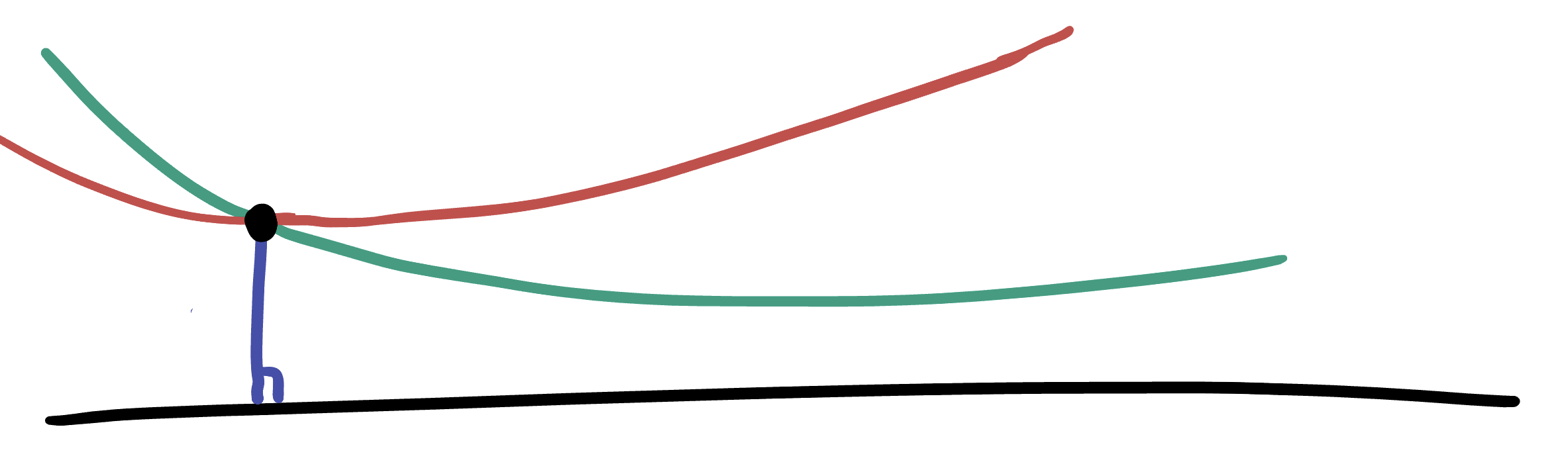
The 5th postulate gives a condition on when two geodesics will intersect: it says if you can measure the angle of intersection they make with a third line, and its less than two right angles, then the two lines intersect one another at some distance along that direction.

Our tool to analyze this situation will be trigonometry, where we’ll reason as follows. Choose some line and pick a point at distance \(d\) away from that line. Through this point, any line we draw makes some angle with the vertical segment of length \(d\), which we can call \(\theta\). Our goal will be to understand how to relate this angle to the point whre the two lines intersect (if they do at all).
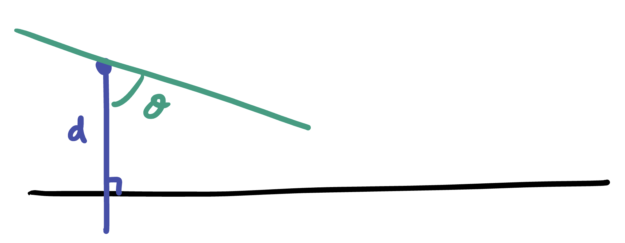
Let’s review first what happens in the Euclidean case. Here, we can use trigonometry to express the relationship between the height \(d\), the angle \(\theta\), and the distance \(L\) to the point of intersection
\[\tan\theta = \frac{L}{d}\]
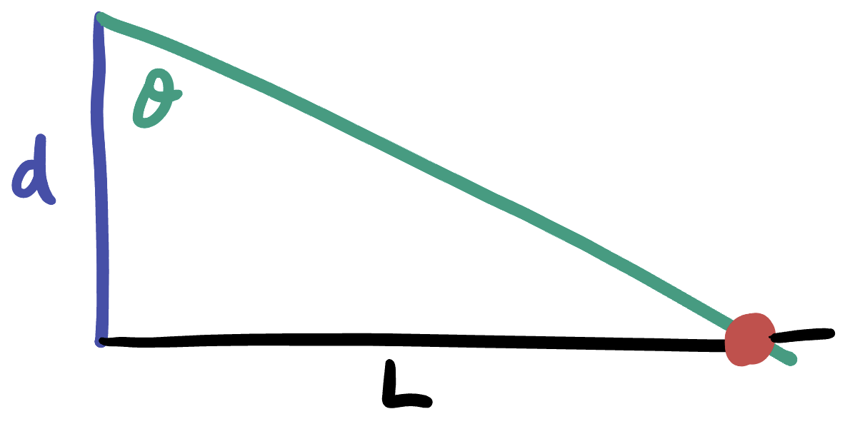
We can then solve this for \(L\), getting \(L=d\tan\theta\). This formula gives us a value for \(L\) any time that \(\tan\theta\) is defined, and so we get a point of intersection whenever \(\theta\neq\pi/2\). When \(\theta=\pi/2\) there is no solution for \(L\), and so there is no point of intersection. Thus, our new line intersects the first except exactly when the sum of the two angles is \(\pi\) (each being \(\pi/2\)), as the parallel postulate states.
What happens to this reasoning if we want to translate it to negatively curved geometry? Well, we will need to figure out what the analogous relationship between \(\theta,d\) and \(L\) should be. While we don’t have any ready-made trigonometric relationship sitting around (yet), we can derive one from what we already know, much like you have done in spherical geometry before:
Exercise 25.19 Using the analogs of right triangle trigonometry in negative curvature, show that
\[\tan\theta = \frac{\tanh L}{\sinh d}\]
Hint: write \(\tan\theta = \sin\theta/cos\theta\), use the fact that we do* know what the trigonometric formulas for sine and cosine should look like (from Example 25.2), and then we also know the pythagorean theorem in negative curvature (Exercise 25.16) to simplify.*
Like in the Euclidean case, we can solve this for \(L\): but perhaps its easier to start by just solving for \(\tanh L\):
\[\tanh L = \sinh d\tan\theta\]
What does this equation tell us? Well, whenever we can find an \(L\) that makes it true that means we have found a point of intersection between our two lines. And, whenever there is no \(L\) which works, we know the two lines do not intersect - they must be parallel! So, analyzing the solutions to this equation will tell us exactly when lines in negative curvature would and would not intersect.
To analyze the possible solutions here, we need to think a bit about the behavior of the hyperbolic-trigonometric that arise. Most importantly, the function$ \(\tanh L\) has horizontal asymptotes at \(\pm 1\), so it is impossible to have any solution to \(\tanh L = x\) if \(|x|\geq 1\).
But wait: it seems pretty easy to make the other side of the equation bigger than 1: both \(\tan\theta\) and \(\sinh d\) are functions that can grow unboundedly! Let’s do an explicit example: if we look at a point \(d=1\) unit of distance away, our equation becomes
\[\sinh(1)\tan\theta \approx 1.175\tan\theta>1\]
This happens anytime \(\tan\theta >1/1.175\approx 0.85\), which is pretty easy to arrange - if \(\theta=0.73\) radians then \(\tan\theta=0.9\) which will do the trick.

But what does this mean? This means that when \(d=1\), the line making angle \(0.73\) with the vertical never manages to intersect the original horizontal line! We have an explicit pair of lines making total angle less than two right angles, whcih nonetheless never intersect one another! Thus, Euclid’s fifth postulate must be false in hyperbolic space!
We can use this same sort of reasoning quickly to see that the equivalent Playfairs axiom is also violated here. Considering the same situation as above, we can take a line, and a point on that line, and find many lines through that point which do not intersect the original: any line making original angle greater than \(\arctan(1/\sinh(1))\) will do!
Thus, our daydreams of pushing the radius past infinity - if they can be formalized - will indeed solve the most important problem of the greeks.