8 Zooming In
8.1 Single-Variable Calculus
Given this new picture of where the infinitesimals of calculus live, its helpful to briefly turn our gaze backwards and consider the calculus we already know in a new light. Instead of drawing a function \(f(x)\) as a graph on \(x\) and \(y\) axes, we will start by thinking of it as a rule, telling us how to move around points on the line. Here’s a depiction of \(y=x^2\) from this perspective.
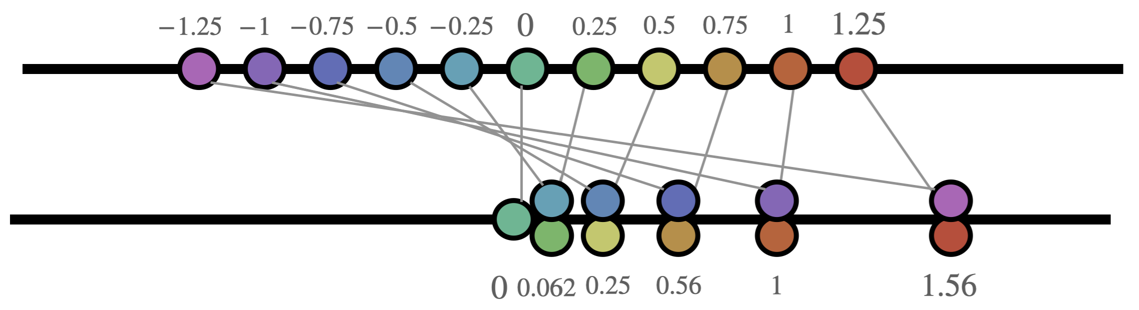
This may be a bit hard to interpret at first, mostly because of all the crossing lines: the squaring operation folds the line in half, sending all the negative numbers to positive numbers, which clutters our view. The same point can be made more clearly with a function that does not do this, such as \(y=x^3\):
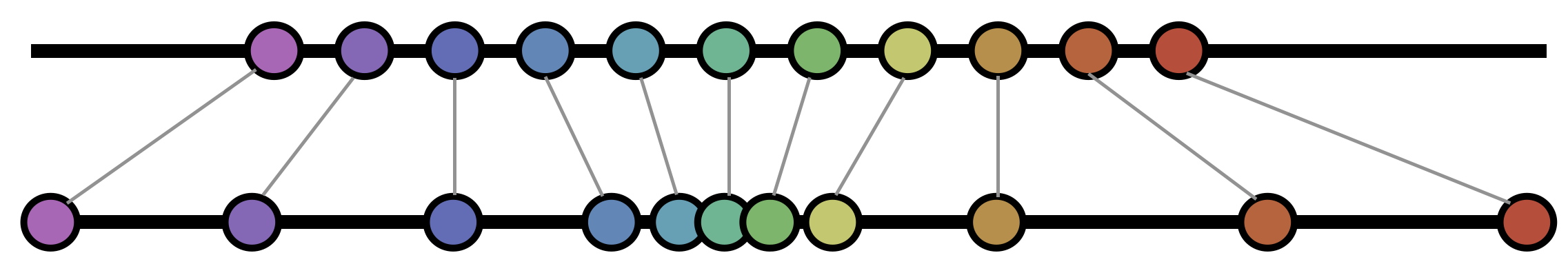
It’s quite easy to see from this map that our function \(f(x)=x^3\) is stretching the line at some points, and compressing it at others. The gray lines connecting inputs to outputs guide our eyes in this qualitative judgement, where we see that points very near the origin are getting pulled closer and closer together, whereas points further out are getting pulled apart.
But this is all an analysis of finite points along the line: what we are really interested in of course, is the infinite level of zoom required by calculus. To see this, we need to imagine the infinitesimal tangent spaces at each point. Below, I’ve illustrated this near a point undergoing infinitesimal stretch, as well as a point undergoing infinitesimal compression.
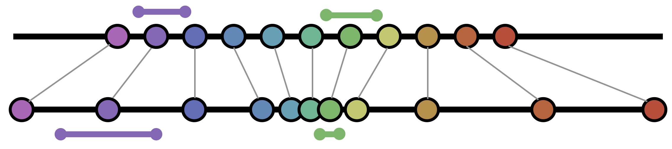
After passing to the tangent space, we expect (via the Fundamental Strategy) that our function becomes a linear function. But the tangent spaces are just lines, and whats a linear map from a line to a line? It’s just multiplication by a constant (a \(1\times 1\) matrix…). Which constant? The derivative, of course! For the example at hand we have
\[f^\prime(x)=3x^2\]
Here we interpret the derivative not as a slope, but as the infinitesimal stretch factor: the fact that \(f^\prime(1)=3\cdot 1^2=3\) means that near the point 1, infinitesimal lengths are being expanded by a factor of 3. The fact that \(f^\prime(0.1)=3\cdot(0.1)^2=0.03\) means that near the point \(1\), distances are stretched by \(0.03\) - that is, compressed by a factor of \(33\)!
It would be great to have a good mental picture of this before we go too far into the weeds. And we are incredibly fortunate that 3Blue1Brown has anticipated our needs, and produced a beautiful video on this topic! This is his final installment in the series “Essence of Calculus”, and while it is the one most relevant to our course (the series focuses on the concepts of Calculus 1 and 2) I wholeheartedly recommend taking some time to refresh your knowledge by watching the entire thing!
8.2 Linearizing Curves
Now we know how to linearize space, how do we find the linearizations of functions at the infinite level of zoom we desire? Its perhaps easiest to start with curves. Curves are functions from some interval \(I\subset \RR\) into \(\RR^2\) or \(\RR^3\). Thus we can write them with components, like \(\gamma(t)=(x(t),y(t))\).
Proposition 8.1 (Differentiating Curves) Let \(\gamma\colon \RR^2\) be a curve. Then at a fixed time \(t\) (and thus a specified point \(\gamma(t)\)), the linearization of the curve is given by the vector \[\gamma^\prime(t)=\lim_{\epsilon\to 0}\frac{\gamma(t+\epsilon)-\gamma(t)}{\epsilon}\] in the tangent space \(T_{\gamma(t)}\RR^2\). If this limit does not exist, the curve is said to be not differentiable at that point.
First, we check that this definition makes sense. If \(\epsilon\) is some small (but finite) number, the points \(\gamma(t+\epsilon)\) and \(\gamma(t)\) are two points along the curve, very near to each other. Their difference is a vector based at \(\gamma(t)\)! Taking the limit as \(\epsilon\to 0\) makes this vector shrink to zero length, but rescaling by \(1/\epsilon\) lets us zoom in, and the result is a *tangent vector based at \(\gamma(t)\)!
Exercise 8.1 Show that if we write the curve \(\gamma(t)=(x(t),y(t))\) in coordinates, that we can use the rules of vector addition and scalar multiplication to simplify this calculation. Indeed, the tangent vector at \(\gamma(t)\) is just given by the derivatives of the coordinate functions \[\gamma^\prime(t)=\langle x^\prime(t),y^\prime(t)\rangle\]
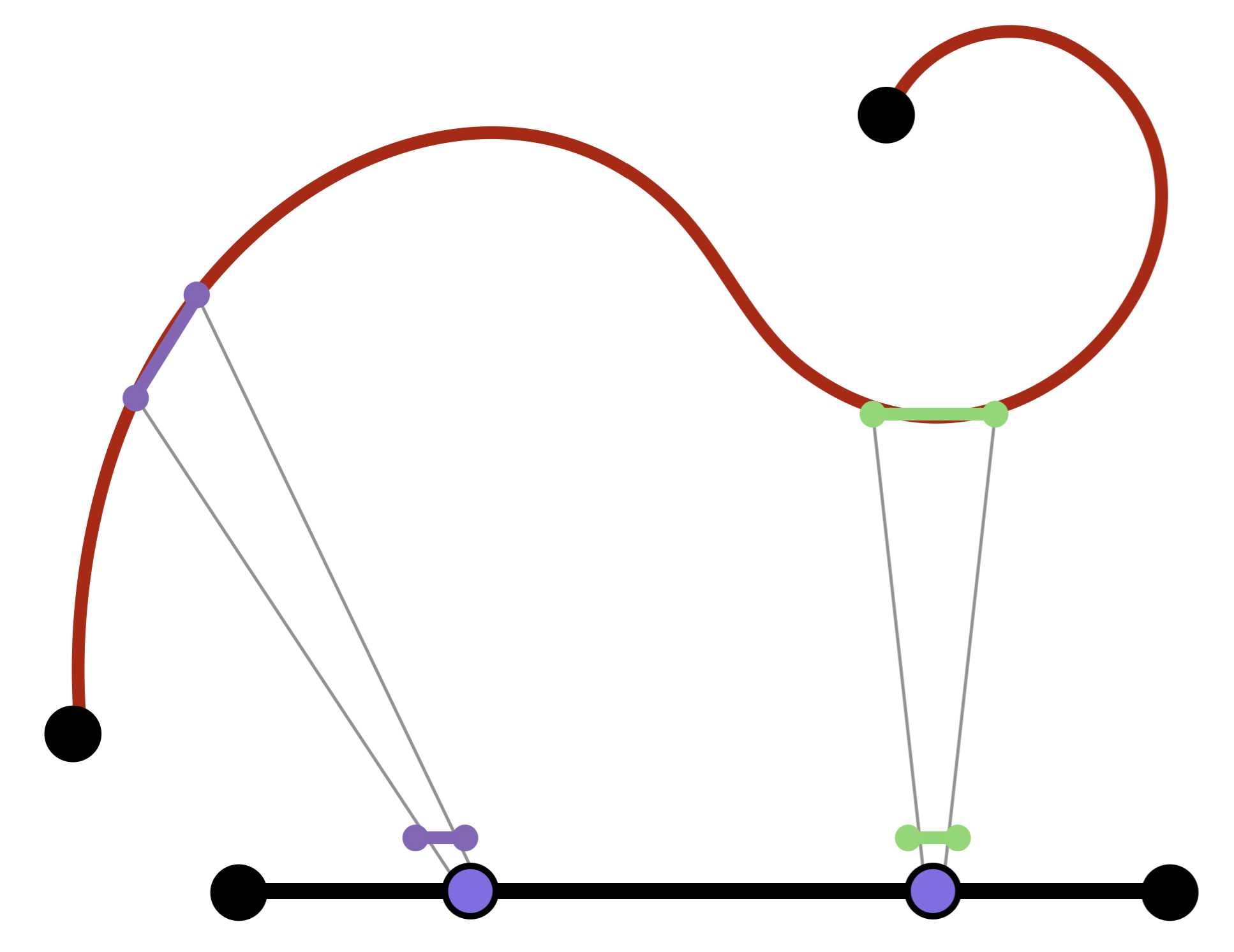
Geometrically, we should interpret this derivative as being a way of taking an infinitesimal piece of the \(t\) line based at the point \(t\), and placing it into the tangent space at \(\gamma(t)\):
Example 8.1 The curve \(f(t)=(t,t^2)\) traces out the standard parabola in the plane. This passes through the point \((2,4)\) when \(t=2\). The derivative of \(f\) is the function \(f^\prime(t)=\langle 1,2t\rangle\), so the tangent vector to \(f\) when \(t=2\) is the vector \[f^\prime(2)=\langle 1, 4\rangle\] in the tangent space \(T_{(2,4)}\RR^2\).
Exercise 8.2 Differentiate the following curves:
- Tangent vector to \((t,\sin(t))\) in \(T_{(\pi/2,1)}\RR^2\).
- Tangent vector to \(f(t)=(\frac{1}{e^t-1},\sqrt{t+1})\) when \(t=2\). Which tangent space is it in?
8.3 Linearizing Multivariable Functions
Besides curves, the other main type of function we will be interested in are functions from a 2-dimensional space back to itself. These are things like rotations of the plane, translations of the plane, but also include even weirder things, that move points about the plane in strange ways.
Definition 8.1 (Multivariable Function) A function \(\phi\) from the plane to itself is a function whose input is a point \(p\in\RR^2\) and its output is another point in the same space: \(\phi(p)\in\RR^2\).
We can make this more concrete by writing both the domain and the range in coordinates: since \(p\in\RR^2\) we can write \(p=(x,y)\) for two numbers \(x,y\). Thus, we can write \(\phi(p)=\phi(x,y)\). But since \(\phi(x,y)\) is also in the plane, we can write it in components as well, say \(\phi(x,y)=(a,b)\). Since the output *depends on \(x,y\) we see that the coordinate \(a\) is a function of both \(x\) and \(y\), as is \(b\). Thus its more helpful to write them as \(a(x,y)\) and \(b(x,y)\) to remember this.
Definition 8.2 If \(\phi\) is a function from the plane to itself, we can write it in components as two separate real-valued functions of \(x\) and \(y\). Often to aid in readability, we name the component functions with the same letter a the overall function: \[\phi(x,y)=\left(\phi_1(x,y),\phi_2(x,y)\right)\]
What should the linearization of such functions look like upon zooming in? Well, we already know how curves work, so a good place to start is by looking for curves. If we hold \(x\) constant in the domain, we get a line parallel to the \(y\) axis through \(p\). Similarly, holding \(y\) constant we get a line parallel to the \(x\) axis through \(P\). Plugging these into \(\phi\), we get two curves passing through \(\phi(p)\).
\[\mathrm{curve_1}(x)=(\phi_1(x,b),\phi_2(x,b)) \] \[ \mathrm{curve_2}(y)=(\phi_1(a,y),\phi_2(a,y))\]

Zooming in, the linearization of these curves are two vectors in \(T_{\phi(p)}\RR^2\), which we can compute explicitly in coordinates:
\[v_x=\mathrm{curve_1}^\prime(x)=\pmat{\frac{\partial}{\partial x}\phi_1(x,b) \\ \frac{\partial}{\partial x}\phi_2(x,b) } \]
\[v_y=\mathrm{curve_2}^\prime(y)=\pmat{\frac{\partial}{\partial y}\phi_1(a,y) \\ \frac{\partial}{\partial y}\phi_2(a,y) } \]
These are each vectors that lie in the tangent space \(T_{\phi(p)}\RR^2\), and so they span a parallelogram there. Indeed, we see that upon zooming in, the map \(\phi\) seems to take an infinitesimal square with sides \(\langle 1,0\rangle\), \(\langle 0,1\rangle\) based at \(T_p\RR^2\) to an infinitesimal parallelogram in the range’s tangent space.
ANIMATION
This is the behavior of a linear map! And even better, we know exactly how to write down a linear map as a matrix if we are given what it does to the standard basis!
Remark 8.1. Here the symbol \(\partial\) denotes a partial derivative: that means, we treat all the other variables as constants, and only differentiate the specified one. It’s easiest to see via example,\(\frac{\partial}{\partial x}(3x^2y+ax+by)=6xy+a+0\) where here we have treated \(y\), \(a\) and \(b\) as constants, and taken only the derivative with respect to \(x\)
Definition 8.3 Let \(\phi\colon \EE^2\to \EE^2\) be a multivariable function, written in components as \[\phi(x,y)=\left(\phi_1(x,y),\phi_2(x,y)\right)\] Then at a point \(p\in\EE^2\), the derivative of \(\phi\) at a point \(p\) is a \(2\times 2\) matrix given by the \(x\) and \(y\) derivatives of its two component functions:
\[D\phi_p = \pmat{\frac{\partial \phi_1}{\partial x} & \frac{\partial \phi_1}{\partial y}\\ \frac{\partial \phi_2}{\partial x} & \frac{\partial \phi_2}{\partial y}}\]
Where after taking the derivatives, we plug in the point \(p\) to each entry of the matrix, to get a matrix of numbers. This is a linear map from the tangent space \(T_p\RR^2\) to the tangent space \(T_{\phi(p)}\RR^2\).
To lighten notation, sometimes we will just write \(\partial_x\) for \(\frac{\partial}{\partial x}\), and we will write a vertical bar for evaluation, much as in calculus:
Example 8.2 The derivative of \(\phi(x,y)=(x+y,\frac{x}{y})\) at the point \((4,7)\) is given by
\[D\phi=\pmat{\partial_x(x+y) &\partial_y(x+y)\\ \partial_x(x/y)&\partial_y(x/y)}=\pmat{1 & 1\\ 1/y & -x/y^2}\]
Plugging in the point,
\[D\phi_{(4,7)}=\pmat{1 & 1\\ 1/y & -x/y^2}\Bigg|_{(4,7)}=\pmat{1&1\\ 1/7 & -4/49}\] Because \(\phi\) takes the point \((4,7)\) to the point \[\phi(4,7)=(4+7,4/7)=(11,4/7)\] this is a linear map from \(T_{(4,7)}\RR^2\) to \(T_{(11,4/7)}\RR^2\)
The usual calculus rules hold: differentiation of a sum of functions is a sum of their derivative matrices, and you can pull scalars out from the derivative
Exercise 8.3 Find the derivatives of the following functions, at the specified points.
- The function \(f(x,y)=(xy,x+y)\) at the point \(p=(1,2)\).
- The function \(\phi(x,y)=\left(xy^2-3x,\frac{x}{y^2+1}\right)\) at the point \(q=(3,0)\).
8.3.1 Compositions
In single variable calculus, we often made use of the chain rule to take derivatives. This let us remember less things, as we were able to construct derivatives of complicated functions from simpler pieces. It’s instructive to take a look back at the formula:
\[(f\circ g(x))^\prime = f^\prime(g(x))g^\prime(x)\]
What is this saying in our new language of linearizations? Recall that the number line itself has tangent spaces, just like the plane, and we should interpret something like \(g^\prime(x)\) as saying the linearization of \(g\) at \(x\). From this perspective, in words this says
The linearization of \(f\circ g\) at \(x\) is the result of linearizing \(g\) at \(x\), and multiplying by the linearization of \(f\) at \(g(x)\).
This makes perfect sense geometrically, where we start with an infinitesimal piece of the line based at \(x\), apply \(g\) so it gets stretched by a factor of \(g^\prime(x)\), and moved to be located at \(g(x)\). Then we apply \(f\): this further stretches by a factor of \(f^\prime(g(x))\)! So the multiplication we see in the formula is really a composition: its saying first stretch by \(g\), and then stretch by \(f\).
This has a direct analog in higher dimensions, if we remember that the way to compose linear transformations is by matrix multiplication.
Proposition 8.2 (Differentiating Compositions) If \(F, G\) are both transformations of the plane, the derivative of \(F\circ G\) at the point \(p\) is the composition of the derivative of \(G\) at \(p\) with the derivative of \(F\) at \(G(p)\):
\[D(F\circ G)_p = DF_{G(p)}DG_p\]
Example 8.3 If \(G(x,y)=(xy,x+y)\) and \(F(x,y)=(2x-y,xy)\) then we compute the derivative of \(F\circ G\) at \((1,2)\) as follows: First, we find the derivative of \(G\) at \((1,2)\): \[DG_{(1,2)}=\pmat{y & x\\1+y &1+x}\Bigg|_{(1,2)}=\pmat{2&1\\ 3&2}\]
Then, since \(G\) takes \((1,2)\) to the point \(G(1,2)=(1\cdot 2, 1+2)=(2,3)\), we need the derivative of \(F\) at \((2,3)\):
\[DF_{(2,3)}=\pmat{2-y&-1\\ y & x}\Bigg|_{(2,3)}=\pmat{-1&-1\\ 3&2}\]
Finally, we compose these linear maps with matrix multiplication (making sure to be careful about the order!)
\[DF_{(2,3)}DG_{(1,2)}=\pmat{-1&-1 \\ 3&2}\pmat{2&1\\ 3&2}=\pmat{-5&-3\\12&7}\]
Exercise 8.4 If \(F,G,H\) are the following multivariate functions \[F(x,y)=(x-y,xy)\] \[G(x,y)=(-y,x)\] \[H(x,y)=(x^3,y^3)\]
Differentiate the following compositions:
- \(F\circ G\) at \((1,1)\)
- \(G\circ G\) at \((0,2)\)
- \(F\circ G\circ H\) at \((-1,3)\).
8.3.2 Inverses
Inverse of \(F\) is a function \(H\) with \(H(F(x))=x\), which ‘undoes’ the action of \(F\) at each point. Familiar one dimensional examples include squaring and the square root, exponentials and logarithms, as well as trigonometric functions and their arc-versions (\(\sin\) and \(\arcsin\) for example). One nice consequence of the chain rules is that it’s possible to differentiate an inverse function, even if you don’t have an explicit formula for it!
The same reasoning applies directly in higher dimensions: if \(F\) is a multivariable function with inverse \(H\), then the composition \(HF=I\) is the identity function, sending every point \(p\) to itself. This is straightforward to differentiate: if \(I(x,y)=(x,y)\) then \[DI = \pmat{\partial_x x &\partial_y x\\ \partial_x y &\partial_y y}=\pmat{1&0\\0&1}\]
Note that the matrix we got by differentiating is constant - it has no \(x\)’s or \(y\)’s in it: thus this matrix represents the derivative of the identity function at every point in the plane. Now, using the multivariate chain rule we can differentiate the equation \(HF=I\) to get
\[D(HF)_a=DH_{F(a)}DF_a=\pmat{1&0\\0&1}\]
But this says that the two matrices, \(DH\) at \(F(a)\) and \(DF\) at \(a\) multiply to give the identity matrix! This is the definition of being inverse matrices, so we have
Theorem 8.1 If \(F\) is an invertible multivarible function, its inverse function \(H\) has the following derivative:
\[DH_{F(a)}=(DF_a)^{-1}\]
Note that this theorem only tells us how to find the derivative at the point \(F(a)\): to find it at a point \(p\) we want, we need to do some more work, and figure out which point \(F\) sends to \(p\).
Example 8.4 Let \(F(x,y)=(x^3,x^2y)\), and let \(H\) be its inverse where defined. To find the derivative of \(H\) at \((8,4)\), we first find the derivative matrix of \(F\) \[DF = \pmat{\partial_x (x^3) & \partial_y (x^3)\\ \partial_x (x^2y) & \partial_y(x^2y)}=\pmat{3x^2 &0\\ 2xy & x^2}\]
Then, we invert this, using the formula for \(2\times 2\) matrix inverses
\[(DF)^{-1}=\frac{1}{3x^2\cdot x^2-0\cdot 2xy}\pmat{x^2 &0\\-2xy & 3x^2}\] \[=\frac{1}{3x^4}\pmat{x^2 &0\\-2xy & 3x^2}\]
By Theorem 8.1, this is the derivative of the inverse \(H\) at the point \(F(x,y)\). We want to find the derivative at \((8,4)\), so we need to know which values of \((x,y)\) to plug in. That is, we need to solve for which \((x,y)\) satisfies \(F(x,y)=(8,4)\). This is a system of equations: \[F(x,y)=\pmat{x^3\\ x^2y}=\pmat{8\\ 4}\] The first equation tells us that \(x=2\), as that’s the only real number that cubes to \(8\). Now we can plug this into the second equation, which says \(2^2y=4\), so \(y=1\). Plugging in \((2,1)\) gives the result
\[DH_{(8,4)}=(DF_{(2,1)})^{-1}=\frac{1}{3\cdot 2^4}\pmat{2^2&0\\ -2\cdot 2\cdot 1 & 3\cdot 2^2}\] \[=\frac{1}{48}\pmat{4&0\\-4&12}\]
As a review of Calculus I, try this out for a function of a single variable yourself:
Exercise 8.5 Consider the function \(f(x)=\arccos(x)\) what is its derivative at \(x=\frac{1}{2}\)?
8.3.3 Differentiating Linear Maps
We won’t actually have that many opportunities during the course where we will need to find the explicit derivatives of an inverse function as we did above. But during the proof of Theorem 8.1, we noticed an interesting fact: the derivative of many maps we have calculated depends on which point \((x,y)\) we were differentiating them at. But not the map \(I(x,y)=(x,y)\): its’ derivative was a constant! If you look at our computation you’ll notice this can certainly be generalized: for instance the derivative of \(f(x,y)=(2x+y,x-y)\) is a constant matrix for the same reason.
Proposition 8.3 (Derivative of a Linear Map) If \(\phi\) is a linear map, then \(D\phi\) is constant, and equal to \(\phi\).
Exercise 8.6 Prove Proposition 8.3.
While the symbolic proof of this is relatively straightforward, its good to pause for a minute and contemplate what it means. The derivative at a point is supposed to be the best linear approximation to the function at that point. But what happens if the function is already linear? Well - then the best linear approximation at that point is itself! And this is true at every point - so the derivative is the same as the map at every point!
In symbols, if \(M\) is a matrix and our linear function is \(f(p)=Mp\), then the derivative is \(Df_p=M\). We ar already very familiar with this from single-variable calculus, although perhaps we did not think through the meaning carefully at the time. After all, what is the derivative of the linear function \(y=mx\)? Its the constant \(y=m\): which is just saying that infinitesimally near every \(x\), the function \(y=mx\) is scaling things up by a factor of \(m\).
Can we characterize which maps have this property? If \(\phi=(\phi_1(x,y),\phi_2(x,y))\), when is it the case that \(D\phi_{(x,y)}\) is a constant matrix?
Exercise 8.7 (When the derivative is constant) Prove that a function \(\phi\colon\RR^2\to\RR^2\) has a constant derivative if and only if the function is affine: that is, a linear map plus constants.