24 Stereographic
In the wake of our proof of the mapmaker’s dilemma, we rise once more to build a map: this time no longer worried about trying to make it optimal in every regard, but just mathematically simple, and easy to interpret.
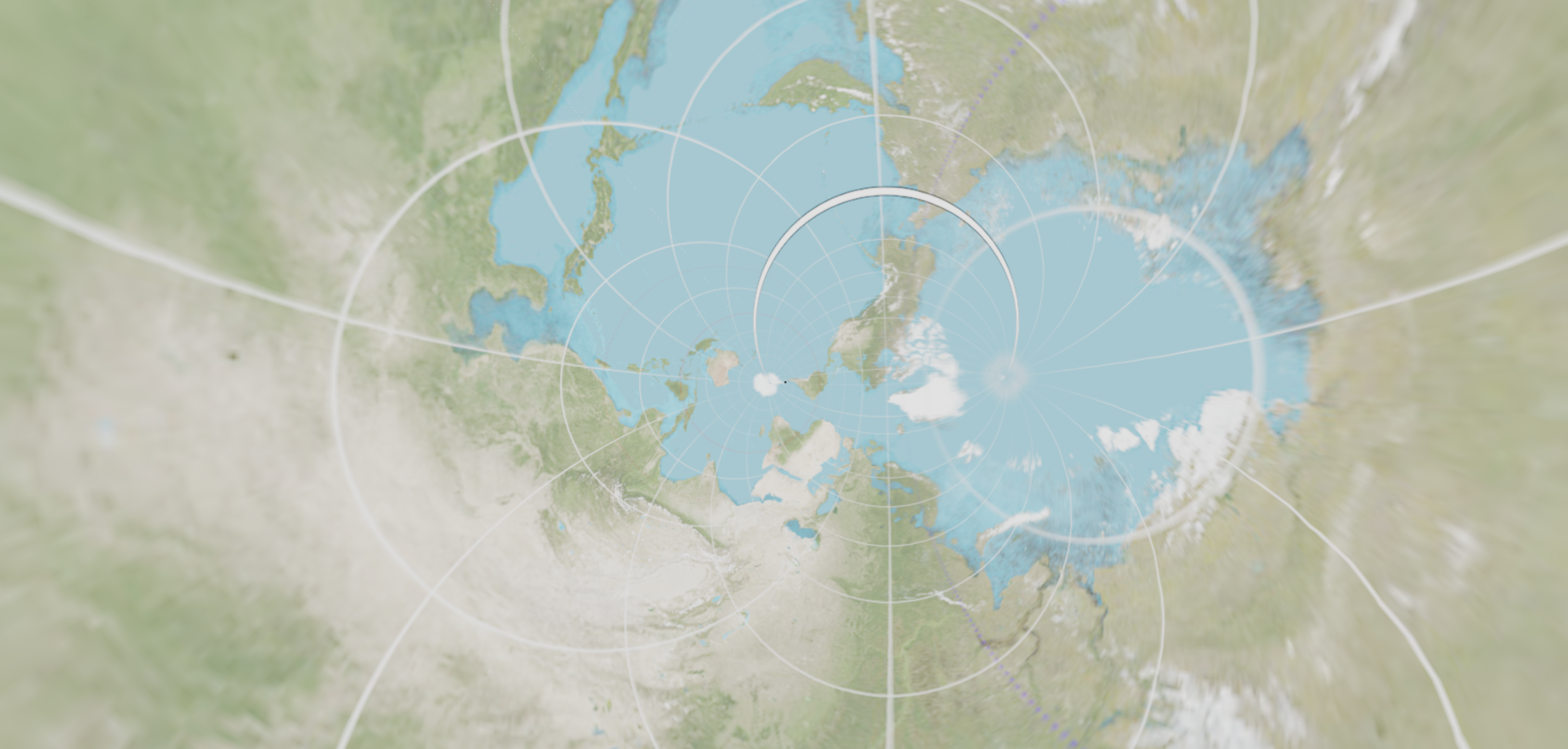
One very natural contender for such a map is stereographic projection first invented by the Greeks to make a star chart, representing the spherical sky on a flat piece of paper. As we’ve come to expect of Greek mathematics, this map has a geometric definition
Definition 24.1 (Stereographic Projection) Given the unit sphere \(\SS^2\) in \(\EE^3\), the stereographic projection of a point \(p\in\SS^2\) is the point \(\sigma(p)\in\EE^2\) such that the straight line in \(\EE^3\) connecting \(p\) to the north pole \(N=(0,0,1)\) intersects the \(xy\) plane in the point \((\sigma(p),0)\).
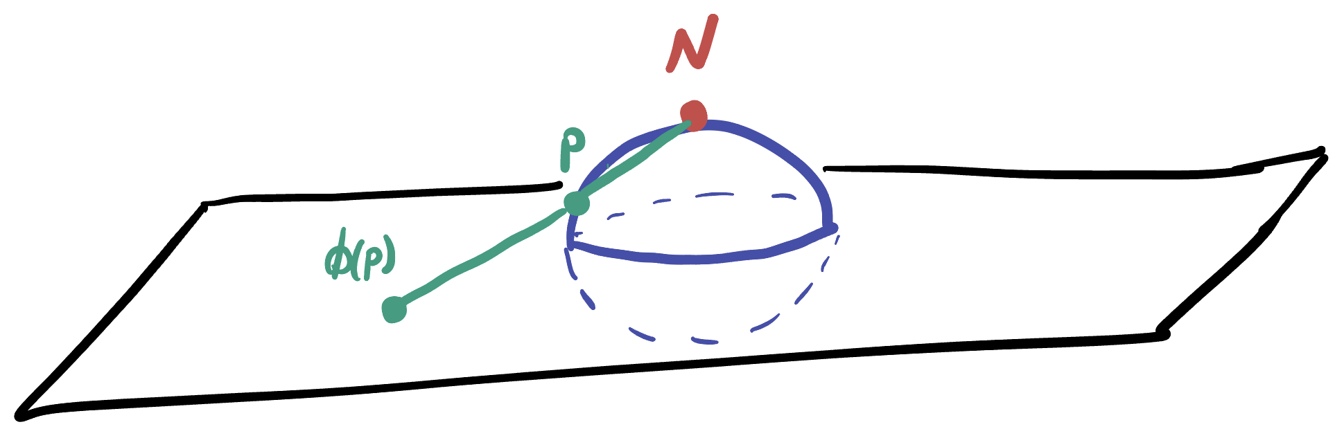
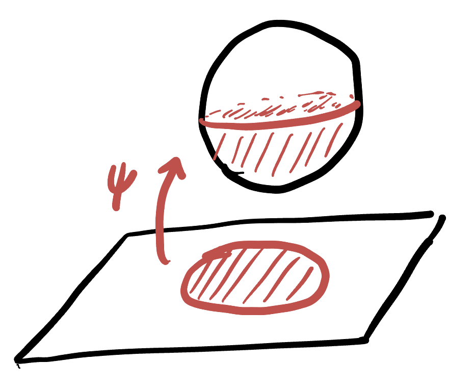
This is much easier to see in three dimensions with an animation than a drawing-by-hand, so here’s one to help (though, in both of these animations I have moved the sphere above the plane: this doesn’t change the math in any essential way but makes things easier to see what is going on)
'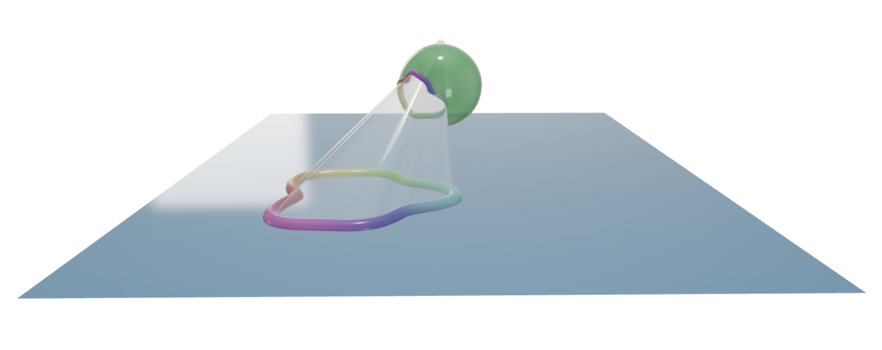
Stereographic projection acts like finding a shadow, from a light source at the top of the sphere.
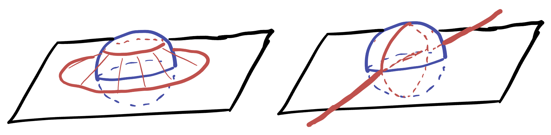
From this picture, we can derive an algebraic formula describing this projection (note that while we have visualized it above as though the sphere is above the plane, the algebra is a bit easier if you assume the plane intersects the sphere in the equator, as in the hand-drawn image above).
Proposition 24.1 (Stereographic Projection Formula) Stereographic projection provides a map of the sphere (except for the north pole), onto the entire Euclidean plane. Its chart is \[\phi(x,y,z)=\left(X,Y\right)=\left(\frac{x}{1-z},\frac{y}{1-z}\right)\]
and the parameterization
\[\psi(X,Y)=(x,y,z)=\left(\frac{2X}{X^2+Y^2+1},\frac{2Y}{X^2+Y^2+1},\frac{X^2+Y^2-1}{X^2+Y^2+1}\right)\]
Proof. We compute the chart, and leave the process of finding its inverse as an exercise. In fact, we can simplify things further by noting that the result must be some multiple of \((x,y)\), as the line connecting \((x,y,z)\) to \((0,0,1)\) in \(\EE^3\) is \((0,0,1)+t(x,y,z-1)\) which projects to \((tx,ty)\) in the plane.
Thus, we can look at the 1D version of the problem, which is the projection of a circle onto the real line through its center, to figure out the scaling factor.

And now we have a problem purely in Euclidean plane geometry, where two similar triangles make an appearance. The result of the mapping takes our point \((x,z)\) to a point distance \(L\) along the real line, so the right triangle with sides \(L\) and \(1\) is similar to the triangle with sides \(L-x\) and \(z\):
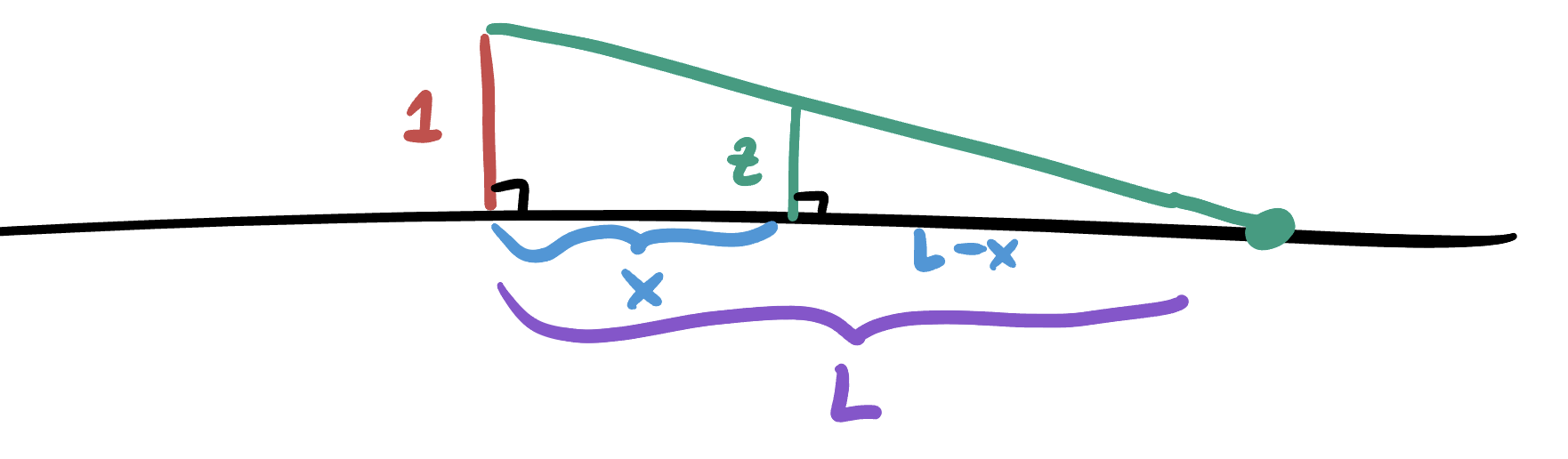
Equating the ratios of the sides gives
\[\frac{L-x}{z}=\frac{L}{1}\]
which simplifies to \(L=\frac{x}{1-z}\). Thus, in general we have
\[\phi(x,y,z)=\left(\frac{x}{1-z},\frac{y}{1-z}\right)\]
Exercise 24.1 Derive the formula for the parameterization associated to stereographic projection, by (1) like above, first focusing on 1 dimension, and then (2) starting with a point \(X\) along the line, solving for the intersection of the line connecting it with \(N\) and the sphere.

This map is very simple algebraically: both the chart and parameterization are given by rational functions (quotients of polynomials). But its also simple geometrically in several particularly nice way, which we explore in the section below.


24.1 Geometry of the Map
Example 24.1 (Equator sent to Unit Circle) Stereographic projection sends the equator of \(\SS^2\) to the unit circle of \(\EE^2\).
We can see this geometrically, as the unit circle already lies in the plane \((x,y,0)\) so by definition stereographic projection doesn’t do anything to it! And, we can see it algebraically, by noting that the \(z\) coordinate of points on the equator is already zero, so \[\phi(x,y,0)=\left(\frac{x}{1-0},\frac{y}{1-0}\right)=(x,y)\]
But this behavior extends beyond the equator to all lines of latitude of the sphere: they are all mapped to circles about the origin in \(\EE^2\)!
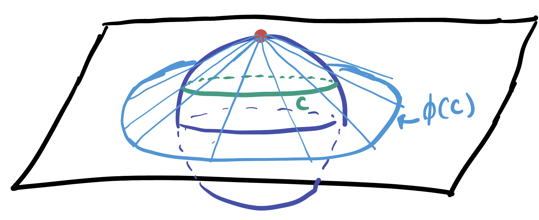
Example 24.2 (Latitudes sent to Circles) Let \(C\) be a circle on \(\SS^2\), centered on the south pole \(S\). Then stereographic projection maps \(C\) to a circle in \(\EE^2\) centered at the origin \(O\).
To see this, note that the circles of \(\SS^2\) centered at one of the poles are contained within a horizontal plane, so the \(z\)-coordinate of all points in \(C\) is constant. Thus after applying \(\phi\) we get
\[\phi(x,y,z)=\left(\frac{x}{1-z},\frac{y}{1-z}\right)=(kx,ky)\] Where \(k=1/(1-z)\) is a constant for all points \(x,y\). Thus the result is just a similarity applied to the original curve \(C\), which was a circle - and similarities take circles to circles!
If we want to be even more precise, we could figure out exactly which circles in the plane they map to.
Exercise 24.2 Let \(C\) be the circle of radius \(r\) about the south pole \(S\) of \(\SS^2\). Show that under stereographic projection the circle this maps to in \(\EE^2\) has Euclidean radius
\[\frac{\sin r}{1+\cos r}\]
Hint: Show the circle centered at \(S\) of radius \(r\) lies in the plane \(z=-\cos r\)…then apply stereographic projection.
The other curves we can understand well are the great circles through the poles.
Example 24.3 (Great Circles through Projection Map to Lines) Each great circle through the poles of \(\SS^2\) projects to a line through the origin.
To see this, we recall that great circles are all contained in a plane through the origin, and so a great circle through the poles is contained in a vertical plane. But the definition of stereographic projection involves drawing lines between \(N\) and points, and for points in a vertical plane, these lines also lie in that same vertical plane! Thus, the projection of this vertical plane is just its intersection with the horizontal plane, which is a straight line through the origin.
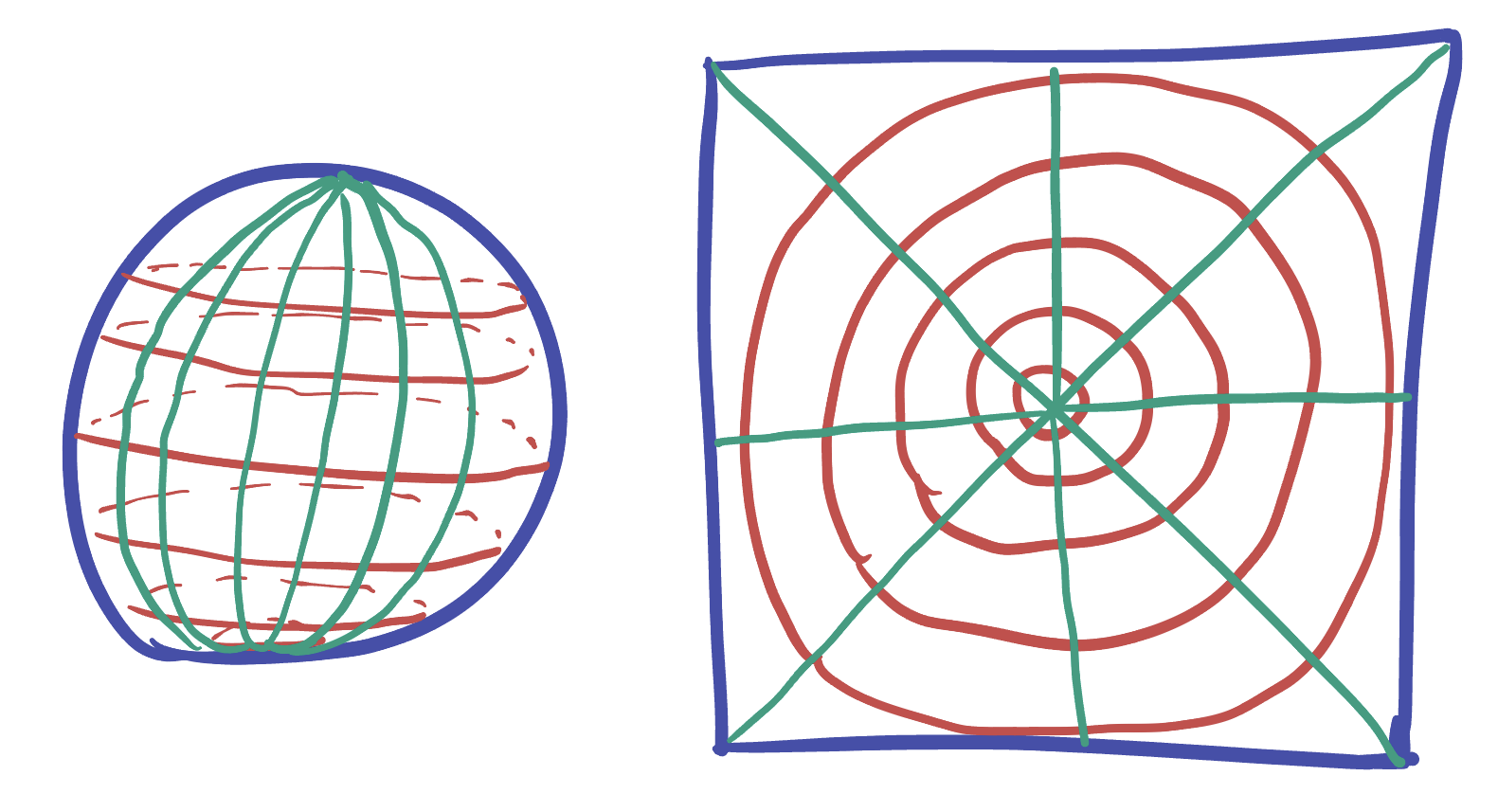
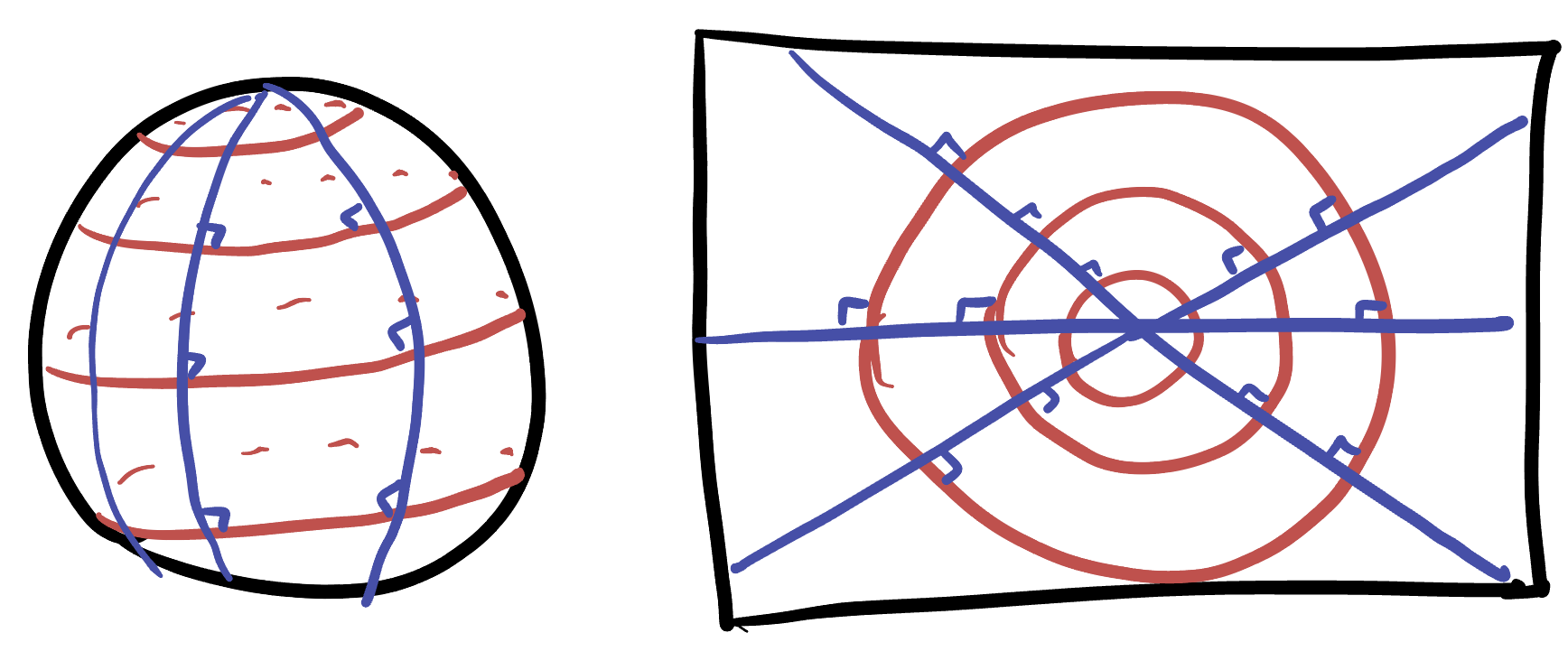
This gives a nice grid on the plane
24.1.1 Generalized Circles
We saw already that great circles through the north pole get mapped to straight lines through the origin int the plane. But this does not mean that all geodesics map to lines, as the equator maps to the unit circle!
But its just just geodesics that map to circles either, we saw that circles around the north and south pole also map to circles in the map. It seems that circles and lines (geodesics) on the sphere are sent to circles and lines on the plane, but they might get mixed up. What a weird property! And one that’s hard to state. So let’s introduce a nice piece of terminology.
Definition 24.2 (Generalized Circle) A generalized circle on the plane is a curve that is either (1) a Euclidean circle, or (2) a Euclidean straight line.

Theorem 24.1 (Stereographic Projection Preserves Generalized Circles) Stereographic projection sends any circle on the sphere to a generalized circle on the plane.
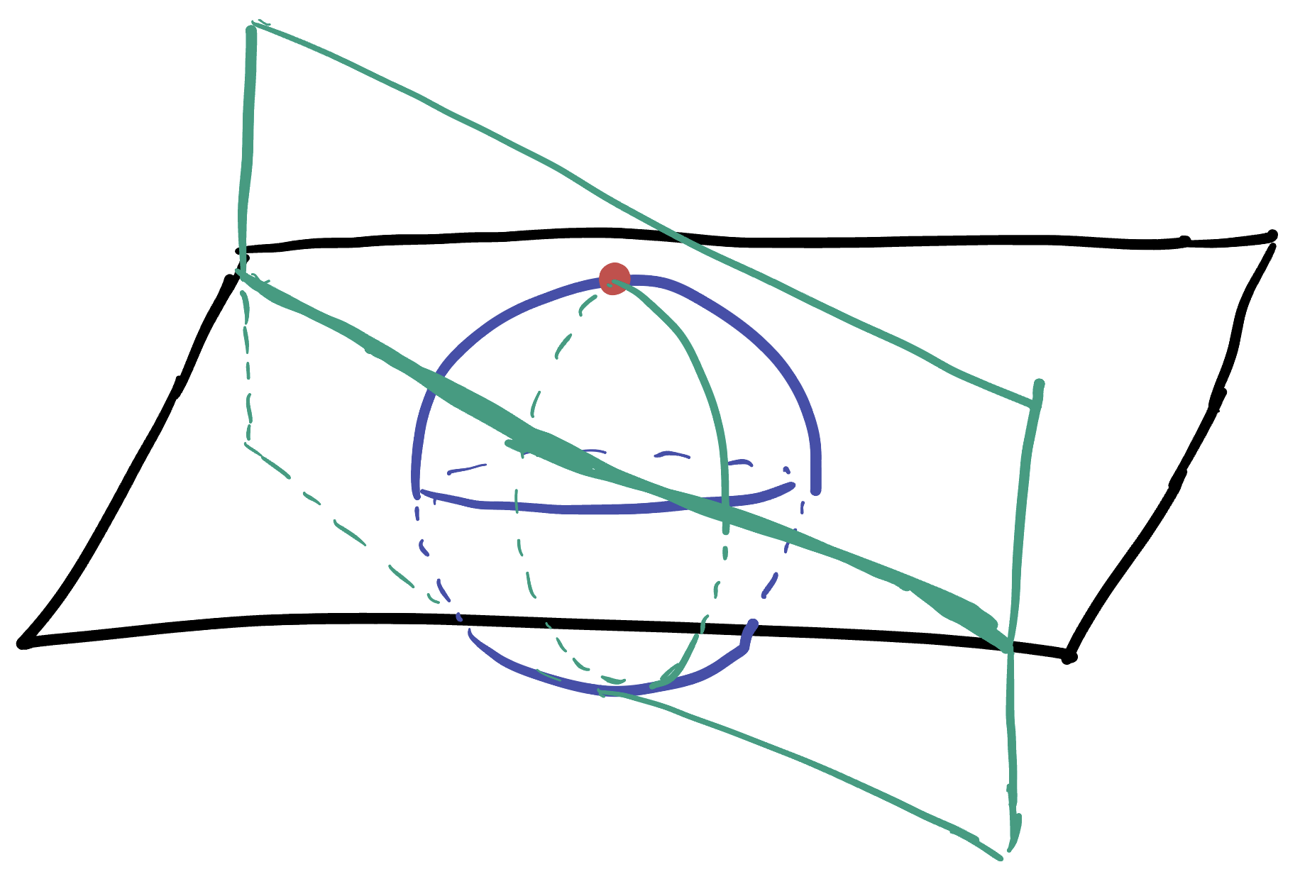
Proof. A circle on \(\SS^2\) is the intersection of the sphere with a plane (when this plane is through the origin, its a great circle, which is also a geodesic). So we are really interested in showing that stereographic projection maps the spots where a plane intersects the sphere to a circle in the plane.
This can be done geometrically, or by an algebraic computation. Here I’ll give the algebra, and below I’ll link to a beautiful visualization of the geometric proof. A plane in \(\EE^3\) is described by an equation of the form
\[ax+by+cz=d\]
But we can use \(\psi\) to express these \(x,y,z\) on the sphere in terms of \((X,Y)\) on the plane:
\[\psi(X,Y)=(x,y,z)=\left(\frac{2X}{X^2+Y^2+1},\frac{2Y}{X^2+Y^2+1},\frac{X^2+Y^2-1}{X^2+Y^2+1}\right)\]
Plugging these in, we see
\[a\frac{2X}{X^2+Y^2+1}+b\frac{2Y}{X^2+Y^2+1}+c\frac{X^2+Y^2-1}{X^2+Y^2+1}=d\]
This looks bad with all the fractions, but we can clear denominators to get
\[2aX+2bY+c(X^2+Y^2-1)=d(X^2+Y^2+1)\]
This still looks pretty bad, but its not really! Let’s collect all the terms with \(x\)’s and \(y\)’s on one side, and group things with similar constants together. \[(c-d)(X^2+Y^2)+2aX+2bY=d+c\]
This is a quadratic equation where \(X^2\) and \(Y^2\) have the same coefficient! That means, this is a circle! (We just need to complete the square if we want to know its center and radius….)
Except…..when that coefficient is equal to zero (when \(c=d\)). Then there are no \(X^2\) or \(Y^2\) terms, and its a linear equation! So intersections of planes with the sphere either map to circles in the plane or to lines in the plane, as required.
24.2 Infinitesimal Geometry
Our main goal of infinitesimal geometry is to show that stereographic projection is conformal: that angles are preserved, and all infinitesimal quantities are controlled by a single scaling factor.
Of course, one means of doing this is brute force calculus: just differentiate the parametrization and compute its action on infinitesimal squares. But with a map as nice as stereographic projection, one can avoid getting so messy with formulas and instead reason more geometrically as well. We shall pursue the geometric approach in this section, though I recommend you work out the calculus-only argument for practice.
The first thing we notice, from our dealings with lines of latitude and longitude above is that these originally orthogonal curves on the sphere are sent to two families of orthogonal curves in the plane. This implies that infinitesimal squares lined up with latitude and longitude to infinitesimal rectangles lined up with circles about \(0\) and lines through \(0\), and vice versa.
To show that the overall map is conformal then, all we need to show is that such an infinitesimal square is stretched the same amount in each of these directions.
Proposition 24.2 (Infinitesimal Angle Length) At a point distance \(r\) from the south pole on \(\SS^2\), the infinitesimal stretch along the circle of latitude containing this point is \[\frac{1}{1+\cos r}\]
Proof. A circle of radius \(r\) on the sphere has circumference \(2\pi\sin r\). This projects to a circle on the plane of Euclidean radius \(\frac{\sin r}{1+\cos r}\), and hence circumference \(2\pi \frac{\sin r}{1+\cos r}\).
The ratio of lengths is the scaling factor: how much the length of the circle was increased or decreased by projection:
\[\frac{2\pi\frac{\sin{r}}{1+\cos r}}{2\pi \sin r}=\frac{1}{1+\cos r}\]
Proposition 24.3 (Infinitesimal Radial Length) At a point distance \(r\) from the south pole on \(\SS^2\), the infinitesimal stretch along the line of longitude containing this point is \[\frac{1}{1+\cos r}\]
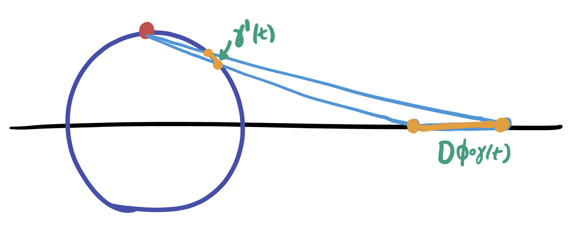
Proof. Here we need only take the derivative along any geodesic through \(S\). One such geodesic is the great circle in the \(xz\) plane \(\gamma(t)=(\sin t, 0,-\cos t)\) which passes through \((0,0,-1)=S\) at \(t=0\). This maps under stereographic projection to
\[\phi(\gamma(t))=\frac{\sin{t}}{1+\cos t}\]
Whose derivative measures the expansion rate of the geodesic as it is mapped onto the plane:
\[\begin{align*}D(\phi\circ\gamma)_t&=\frac{\cos t(1+\cos t)-\sin t(-\sin t)}{(1+\cos t)^2}\\ &=\frac{\cos t + \cos^2 t+\sin^2 t}{(1+\cos t)^2}\\ &=\frac{1+\cos t}{(1+\cos t)^2}\\ &=\frac{1}{1+\cos t} \end{align*}\]
Thus at distance \(r\) away from the center (so \(t=r\) as the unit circle is a unit-speed curve), the rate of stretching rate is
\[\frac{1}{1+\cos r}\]
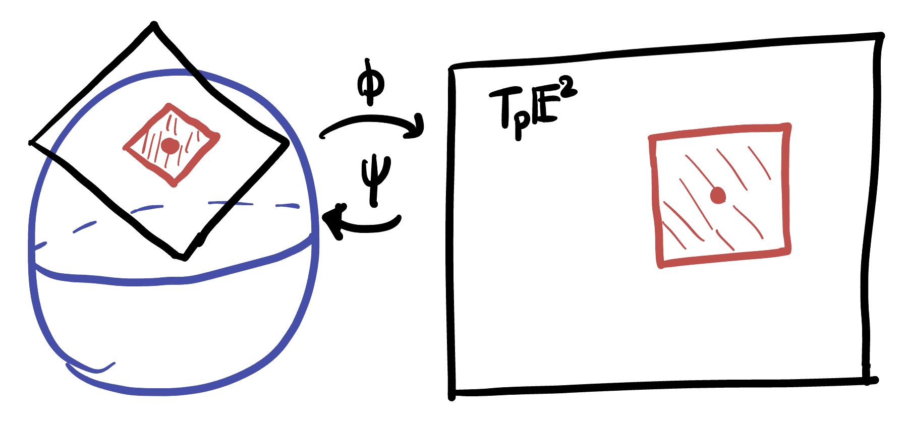
The two thereoms above tell us that at any point of the sphere, the latitude and longitude directions are both stretched by the same factor! This means that infinitesimal squares in \(T_p\SS^2\) are mapped to infinitesimal squares
Theorem 24.2 (Stereographic Projection is Conformal) Stereographic projection preserves angles: it sends infinitesimal squares to infinitesimal squares.
Proof. At any point \(p\), the stereographic projection chart the curve of longitude and latitude through \(p\) to orthogonal curves on the plane. It stretches each of these curves by the same factor, \(1/(1+\cos r)\), meaning that it takes a unit square in \(T_p\SS^2\) to a square of side length \(1/(1+\cos r)\) in \(T_{\phi(p)}M\).
Thus, \(\phi\) takes infinitesimal squares to other infinitesimal squares! This means (by the discussion in the angle chapter) that \(\phi\) preserves all angles, so \(\phi\) is a conformal map.
Now that we know that stereographic projection is conformal, we know it stretches all vectors by the same amount at a given point. Our calculations above confirmed this fact using the chart, but most interesting calculations we will want to do need the parameterization.
Exercise 24.3 (Stereographic Map-Coordinates) The fact that stereographic projection is conformal means that at a given point \(p=(X,Y)\) in \(\EE^2\), the parameterization \(\psi\) must stretch all vectors by the same amount. By applying \(D\psi\) to a vector, calculate this amount and show it to be \[\frac{2}{1+X^2+Y^2}\]
Because all vectors are stretched in the same way, we can write down the map dot product easily: after a little calculation we see it is just a multiple of the Euclidean dot product on the plane!
Theorem 24.3 (Stereographic Dot Product) Let \(p=(X,Y)\) be a point in the plane, and \(v=\langle v_1,v_2\rangle\), and \(w=\langle w_1,w_2\rangle\) be two vectors in \(T_p\EE^2\). Their map dot product is
\[(v\cdot w)_\map = (D\psi_p v)\cdot (D\psi_p w)= \frac{4}{(1+X^2+Y^2)^2}(v\cdot w)\]
Proof. Let \(e_1=\langle 1,0\rangle\) and \(e_2=\langle 0,1\rangle\) to help with notation. Then we can write \(v\) as a linear combination of this basis:
\[v=\langle v_1,v_2\rangle = v_1\langle 1,0\rangle+v_2\langle 0,1\rangle = v_1e_2+v_2e_2\]
and similarly for \(w\). Next, using the fact that the derivative is a linear map (its a matrix, after all) we can distribute, and pull out the scalars \(v_i\) and \(w_i\):
\[\begin{align*}D\psi_p(v)&=D\psi_p(v_1e_2+v_2e_2)\\ &= D\psi_p(v_1e_)+D\psi_p(v_2e_2)\\ &=v_1D\psi_p(e_1)+v_2D\psi_p(e_2) \end{align*}\]
and again, similarly for \(w\). Now we wish to compute the dot product, so we multiply it all out:
\[\begin{align*} (D\psi_p v)\cdot (D\psi_p w)&=(v_1D\psi_p e_1+v_2D\psi_p e_2)\cdot (w_1D\psi_p e_1+w_2D\psi_p e_2)\\ &= v_1w_1(D\psi_p e_1)\cdot (D\psi_p e_1)+ v_1w_2 (D\psi_p e_1)\cdot (D\psi_p e_2)\\ &+v_2w_1 (D\psi_p e_2)\cdot (D\psi_p e_1)+w_1w_2 (D\psi_p e_2)\cdot (D\psi_p e_2) \end{align*}\]
Now we have to think a bit about what we know! Since \(\psi\) does not change angles, and \(e_1\) and \(e_2\) are orthogonal, we know that \(D\psi_p e_1\) and \(D\psi_p e_2\) are orthogonal to one another. Thus, their dot product is equal to zero! This gets rid completely of the two middle terms in our big expression, and so we are only left with the first term and the last term.
But both of these are involve the dot product of a vector with itself: like \((D\psi_p e_1)\cdot(D\psi_p e_1)\). This is the definition of the squared length of that vector, but we know exactly how stereographic projection changes lengths! Thus for both \(e_1\) and \(e_2\) we know
\[(D\psi_p e_i)\cdot(D\psi_p e_i)=\left(\frac{2}{1+X^2+Y^2}\right)^2=\frac{4}{(1+X^2+Y^2)^2}\]
Now we putting this all together, we find
\[\begin{align*}(v\cdot w)_\map &= \frac{4}{(1+X^2+Y^2)^2}v_1w_2+0v_1w_2+0v_2w_1+\frac{4}{(1+x^2+y^2)^2}v_2w_2\\ &=\frac{4}{(1+X^2+Y^2)^2}\left(v_1w_2+v_2w_2\right)\\ &= \frac{4}{(1+X^2+Y^2)^2}(v\cdot w) \end{align*}\]
Definition 24.3 (Stereographic Metric) The dot product on \(\EE^2\) given at the point \(p=(X,Y)\) by \[(v\cdot w)_\map = \frac{4}{(1+X^2+Y^2)^2} (v_1w_1+v_2w_2)\]
Is called the stereographic metric.
Using this, we can compute any quantity we may care about on the sphere, using only coordinates of the plane. For instance, the spherical length of a vector is just
\[\|v\|_\map = \sqrt{(v\cdot v)_\map}=\frac{2}{1+X^2+Y^2}\|v\|\]
The area of an infinitesimal piece of the sphere is
\[dA =\left(\langle 1,0\rangle\cdot \langle 0,1\rangle\right)_\map dXdY = \frac{4}{(1+X^2+Y^2)}dXdY\]
etc.
24.2.1 The Disk and Half Plane
One use of stereographic projection is to write down a map of the sphere, as we’ve seen above. But it is also used a lot in mathematics as a tool to help create new and useful functions that would otherwise be difficult to guess. It shows up in this context in applications across geometry, complex analysis, and other fields of math because its conformal, and so we know when building things with stereographic projection as one of the components, it is not going to mess up any angle measures.
Here, we will look at a fundamental example of this, and will use stereographic projection to write down a conformal map which takes points in the unit disk \(x^2+y^2<1\) to the upper half plane \(y\geq 0\) in \(\EE^2\). This map becomes very important in the study of hyperbolic geometry, where we can use it to help us relate two different maps of the mysterious hyperbolic plane.
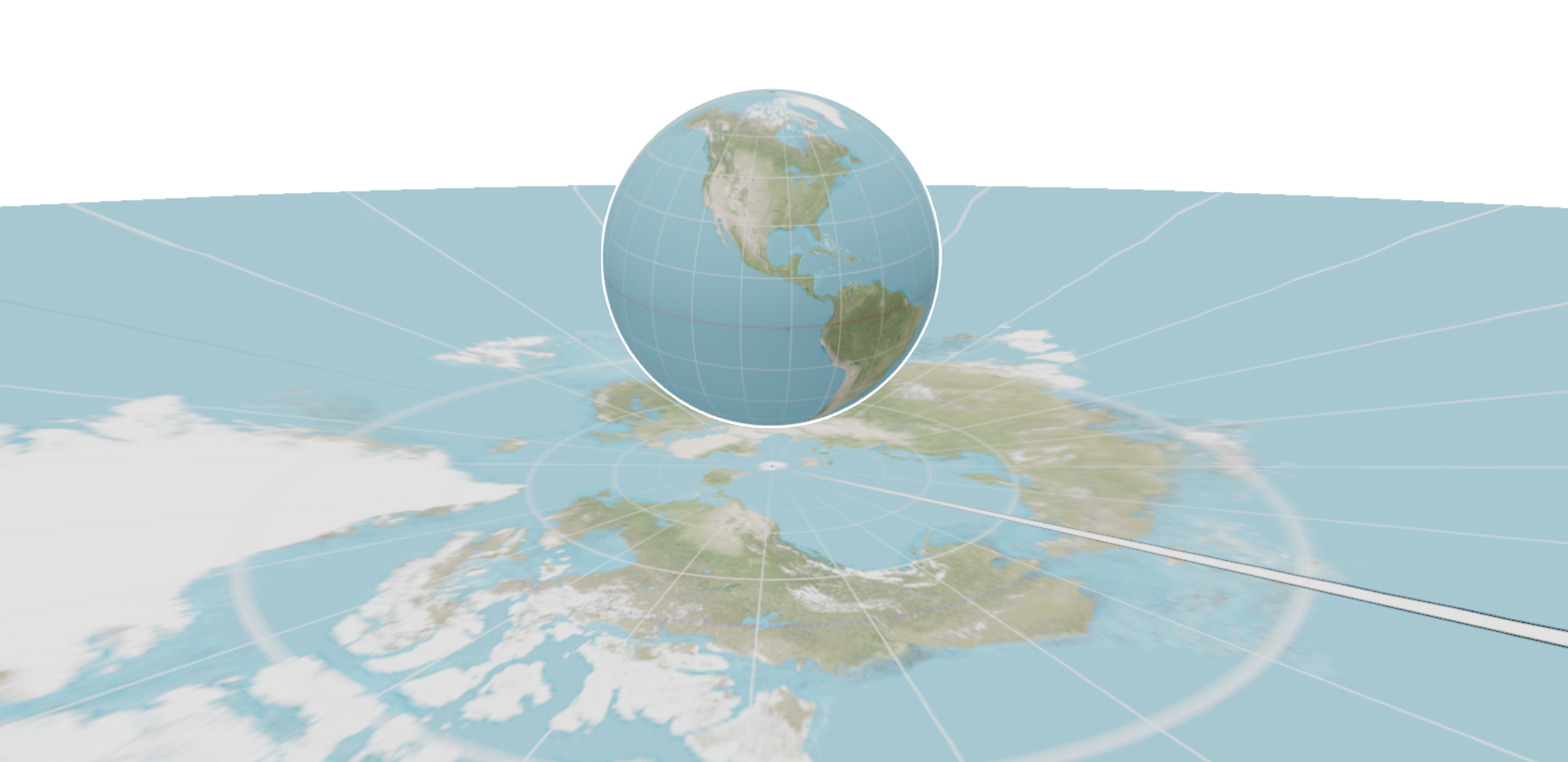
Here’s the idea: starting with the unit disk in the plane centered at \(O\), we can use the parameterization of stereographic projection to map this onto the sphere. Doing so moves the region onto the entire southern hemisphere of \(\SS^2\) (since the unit circle maps to the equator):
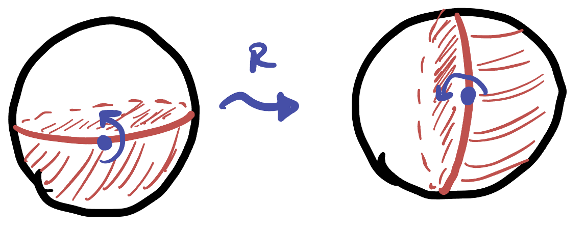
Now, we can rotate the sphere a quarter of a turn about the \(x\)-axis, so that the equator becomes a line of longitude, now passing through the north and south pole, and what was the southern hemisphere is now the positive \(y\) hemisphere: the south pole has been moved to \((0,1,0)\). (How do we write down a rotation about the \(x\) axis? Well, its going to fix the x direction so we know the first column. Then, the second and third column will be where the \(y\) and \(z\) basis vectors go under a quarter turn)
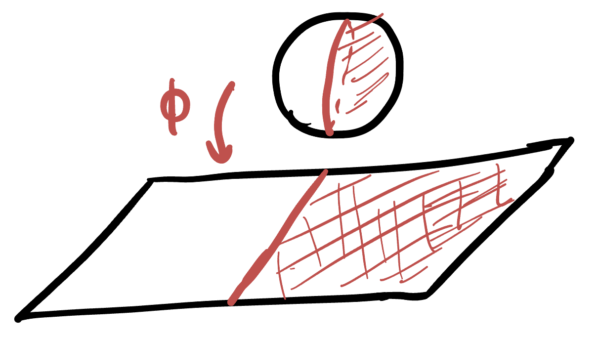
And finally, we can use the chart of stereographic projection to re-project this down onto the plane. Now, the great circle bounding it passes through the north pole, so it projects to a line: the \(x\)-axis! This divided the sphere in two, and so its image divides the plane in two, with our positive \(y\) hemisphere becoming the positive \(y\) half-plane.
Exercise 24.4 (Disk and Half Plane: Construction) Let \(\DD\) be the unit disk \(\DD=\{(x,y)\mid x^2+y^2<1\}\) and let \(\mathbb{U}\) be the upper half plane \(\mathbb{U}=\{(x,y)\mid y>0\}\). Let \(T\colon \DD\to \mathbb{U}\) be the map described above. Prove that $T can be expressed as
\[T(x,y)=\left(\frac{2x}{1+x^2+y^2-2y},\frac{1-x^2-y^2}{1+x^2+y^2-2y}\right)\]
By building it step by step: applying \(\psi\) to get the disk onto the sphere, rotating by the correct quarter turn about the \(x\)-axis, and then applying \(\phi\) to return to the plane.
This map is conformal - meaning that it preserves all angles! And even more than that, it takes generalized circles to generalized circles.
Exercise 24.5 (Disk and Half Plane: Understanding) Prove that these claims are in fact true: that our new function is conformal, and sends generalized circles to generalized circles. Hint: what kinds of maps is it built out of? What do each of these maps to do angles, or to generalized circles (on the plane) / circles (on the sphere)?
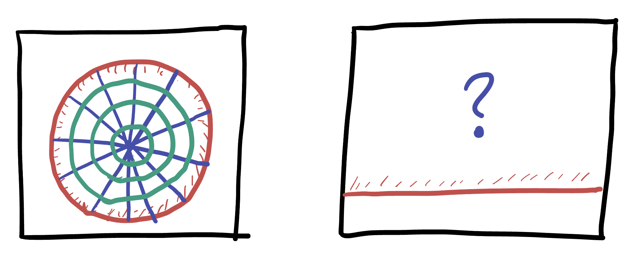
Use this to “transfer” this picture of polar coordinates in the unit disk onto the plane, via our new map.
24.3 The Sphere of Radius \(R\)
Throughout this chapter we have studied stereographic projection in detail, but on the unit sphere. It is not too hard to generalize what we have done to spheres of other radii, and while this may not sound super exciting at first, it actually turns out to be absolutely fundamental to how we are going to discover hyperbolic space! So, it is a rather important exercise to work this all out for yourself.
The good news is you have this entire chapter as a guide, where I’ve worked out many of the details for the case of the unit sphere. The formulas will be quite similar, but there’ll be \(R\)’s inserted in various places: so the second piece of good news is that I’ll give you the formulas that you need to derive! That way, you can check your work.
Definition 24.4 Let \(\SS^2_R\) be the sphere of radius \(R\) in \(\EE^3\). Then the chart \(\phi\) for stereographic projection of this sphere is defined geometrically exactly as in the original version: given a point \(p\in\SS^2_R\), \(\phi(p)\) is where the line connecting \(p\) to the north pole \(N=(0,0,R)\) intersects the \(xy\) plane.
Exercise 24.6 Show that the formulas for both the chart and the parameterization of stereographic projection here are as follows:
\[\phi(x,y,z)=(X,Y)=\left(\frac{Rx}{R-z},\frac{Ry}{R-z}\right)\]
\[\psi(X,Y)=(x,y,z)=\left(\frac{2R^2 X}{X^2+Y^2+R^2},\frac{2R^2 Y}{X^2+Y^2+R^2},R\frac{X^2+Y^2-R^2}{X^2+Y^2+R^2}\right)\]
(It might help to look back at Proposition 24.1, and attempt Exercise 24.1).
Running through the same arguments as in the chapter above (which you don’t have to write down), its straightforward to check that this new map is a conformal map between \(\SS^2_R\) minus \(N\), and the plane. This means its parameterization \(\psi\) both preserves angles and stretches all vectors by a uniform length: we can use this fact to compute the dot product for this map.
Exercise 24.7 At a point \(p=(X,Y)\) on the plane, what is the factor by which a vector \(v\in T_p\EE^2\) is stretched when mapped onto \(\SS^2_R\) by the parameterization of stereographic projection? Hint: we know the factor is the same for all vectors: so pick an easy vector to calculate with and find its length!
Once you know this, follow the argument style of Theorem 24.3 to compute the map-dot product on the plane, and show that it is equal to
\[(v\cdot w)_\map = \frac{4R^4}{(R^2+X^2+Y^2)^2}(v\cdot w)\]