11 Isometries
Besides measuring distance, one of the other most fundamental notions to geometry is that of an isometry, or a rigid motion of space. This comes from greek meaning same-measure, as an isometry is a function that does not change lengths.
Definition 11.1 (Isometries in \(\EE^2\)) An isometry of \(\EE^2\) is a function \(\phi\colon \EE^2\to\EE^2\) which preserves all infinitesimal lengths of \(\EE^2\).
What does it mean to preserve infinitesimal lengths? If \(v\in T_p\EE^2\) is a vector (an infinitesimal segment of a curve), then while \(\phi\) takes \(p\) to a new point \(\phi(p)\), infinitesimally it acts as a linear transformation from \(T_p\EE^2\) to \(T_{\phi(p)}\EE^2\). That infinitesimal linear transformation is the derivative matrix \(D\phi_p\), which takes the original vector \(v\) to \(D\phi_p(v)\). What we are interested in is whether or not \(D\phi_p\) changed the length of \(v\).

Definition 11.2 A function \(\phi\colon \EE^2\to\EE^2\) preserves infinitesimal lengths if for every \(p\in\EE^2\) and every \(v\in T_p\EE^2\), we have
\[\|v\|=\|D\phi_p(v)\|\]
Using this condition, one can show with some calculus that every isometry is actually an invertible function: that means, if \(\phi\) is an isometry there is a function \(\phi^{-1}\) which undoes the action of \(\phi\). We will not prove this theorem here (as it is purely a result of advanced calculus, and doesn’t help us learn geometry). If you like, you can think of this as an extra condition we are assuming* about isometries in this course.
Theorem 11.1 (Isometries are Invertible Functions)
Just as one can apply an isometry to points, one can apply it to an entire curve by composition: if \(\gamma\) is a curve, the curve \(\phi\circ\gamma\) can be thought of as drawing \(\gamma\), and then performing whatever action \(\phi\) specifies.
Theorem 11.2 (Isometries Preserve Lengths of Curves) Let \(\phi\colon\EE^2\to\EE^2\) be an isometry, and \(\gamma\colon I\to \EE^2\) a curve. Then \[\len(\gamma)=\len(\phi\circ\gamma)\]
Proof. Let \(\phi\) be an isometry, and \(\gamma\colon [a,b]\to\EE^2\) be a curve. Then we know the length of \(\gamma\) itself is defined as \(\len(\gamma)=\int_{[a,b]}\|\gamma^\prime(t)\|dt\), and we wish to compare this with the length of \(\phi\circ\gamma\)
\[\len(\phi\circ\gamma)=\int_{[a,b]}\|(\phi\circ\gamma)^\prime(t)\|dt\]
To compute this integral we need to first differentiate \(\phi\circ\gamma\) using the chain rule: \[(\phi\circ\gamma)^\prime(t)= D\phi_{\gamma(t)}\gamma^\prime(t)\] Where here recall that \(D\phi_{\gamma(t)}\) is a matrix - the linear transformation recording the infinitesimal behavior of \(\phi\) at a point - and \(\gamma^\prime(t)\) is a tangent vector - an infinitesimal piece of arc. Since we have assumed that \(\phi\) is an isometry, it preserves infinitesimal lengths by definition so \[\|D\phi_{\gamma(t)}\gamma^\prime(t)\|=\|\gamma^\prime(t)\|\] Using this, we can simplify our integral:
\[\begin{align*} \len(\phi\circ\gamma)&=\int_{[a,b]}\|(\phi\circ\gamma)^\prime(t)\|dt\\ &=\int_{[a,b]}\|D\phi_{\gamma(t)}\gamma^\prime(t)\|dt\\ &=\int_{[a,b]}\|\gamma^\prime(t)\|dt\\ &=\len(\gamma) \end{align*}\]
In fact, the converse of this is true as well: if a differentiable function preserves the lengths of all curves, then it preserves infinitesimal lengths, and is an isometry.
11.1 Translations & Some Rotations
We will go more in-depth in our discussion of isometries later on, but for now it’s good practice with the definition to find a couple examples that we can use.
Theorem 11.3 (Translations are Isometries) If \(v=\langle a,b\rangle\) is a fixed vector, a translation by \(v\) of \(\EE^2\) is given by the function \(T(p)=p+v\), or, in coordinates, \[T(x,y)=(x+a,y+b)\]. This is an isometry of \(\EE^2\).
![]()
Proof. Here we need to compute the derivative of \(T\): Since \(T(x,y)=(x+a,y+b)\) we get the matrix
\[\begin{align*}DT &= \begin{pmatrix}\partial_x T_1& \partial_y T_1\\ \partial_x T_2 &\partial_y T_2\end{pmatrix}\\&=\begin{pmatrix} \partial_x(x+a)&\partial_y(x+a)\\ \partial_x(y+b)&\partial_y(y+b) \end{pmatrix}\\ &= \begin{pmatrix} 1&0\\0&1\end{pmatrix} \end{align*}\]
This is the identity matrix which means it does nothing to vectors: if \(v=\langle v_1,v_2\rangle\) is any vector based at \(p\in\EE^2\) then
\[DT_p(v)=\pmat{1&0\\ 0&1}\pmat{ v_1\\ v_2}=\pmat{v_1\\ v_2}\]
Thus, since \(DT\) did not change anything at all about \(v\) it did not change its length and so \(T\) is an isometry.
\[\|DT_p(v)\|=\|v\|\]
A particularly nice collection of functions to work with are the linear maps \(\EE^2\to\EE^2\). One of the nicest properties of these they are easy to differentiate: recall that if \(A\) is a matrix representing the linear map \(\phi(v)=Av\) then \(D\phi=A\) is the same matrix! So, if we are looking for linear isometries we can save ourselves the work of differentiation.
Example 11.1 The following linear map is an isometry of \(\EE^2\) \[\phi(x,y)=\pmat{0&-1\\1&0}\pmat{x\\ y}\]

Proof. We check that this preserves all infinitesimal lengths. Denote by \(A\) the matrix \(A=\smat{0& -1\\ 1 &0}\), then \(\phi\) is the linear map \(\phi(x)=Ax\), so its derivative is given by the same linear map, \(D\phi_p(v)=Av\) at every point \(p\).
Thus, to see that \(\phi\) is an isometry, all we need to do is check whether or not the length of \(Av\) is the same as the length of \(v\) for an arbitrary vector \(v=\langle v_1,v_2\rangle\).
\[Av=\pmat{0 & -1\\ 1&0}\pmat{v_1\\ v_2}=\pmat{-v_2\\ v_1}\]
\[\begin{align*}\|Av\|&=\|\langle -v_2,v_1\rangle\|\\ &=\sqrt{(-v_2)^2+(v_1)^2}\\ &=\sqrt{v_1^2+v_2^2}\\ &=\|v\| \end{align*}\] As these lengths are the same, \(\phi\) is an isometry.
Of course, not all linear maps are isometries: its easy to cook up something that doesn’t preserve infinitesimal lengths.
Example 11.2 The following linear map is not an isometry of \(\EE^2\): \[\phi(x,y)=\pmat{2&1\\1&0}\pmat{x\\ y}\]
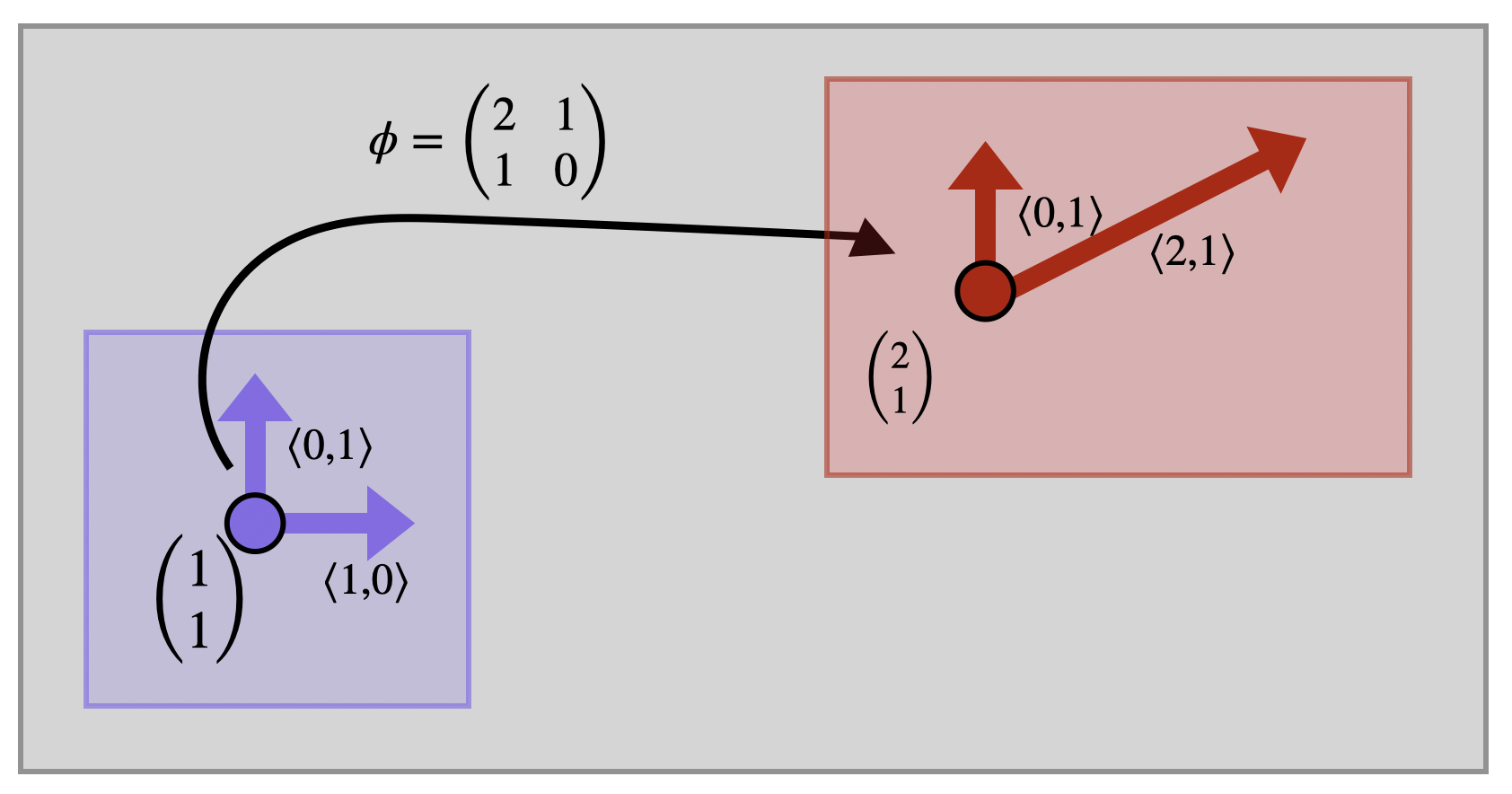
Proof. Since \(\phi\) is linear, \(D\phi\) is equal to the same linear map \(\smat{2 ^1\\ 1&0}\) at each point of \(\EE^2\). To prove \(\phi\) is not an isometry, all we need to do is find one vector which has its length changed by \(D\phi\). Consider the vector \(v=\langle 1,0\rangle\) based at \(p=O\in\EE^2\). Then
\[D\phi_p(v) = \pmat{ 2&1 \\ 1&0}\pmat{1\\ 0}=\pmat{2\\ 0}\]
While \(v\) had unit length \(D\phi_p(v)\) has length \(2\), so \(\phi\) does not preserve all infinitesimal lengths, and therefore is not an isometry.
What are the conditions on a linear map being an isometry? Well, if it needs to preserve all infinitesimal lengths, it needs to send the unit vector \(\langle 1,0\rangle\) to some other unit vector, and same for \(\langle 0,1\rangle\). Since the image of these vectors are the first and second columns of the matrix representing them, this means that every linear isometry has a matrix whose rows are unit vectors. Is every such matrix an isometry?
Exercise 11.1 Write down a linear map that sends both \(\langle 1,0\rangle\) and \(\langle 0,1\rangle\) to unit vectors, but is not an isometry.
However, if we choose unit vectors correctly, we do get an linear isometry! Intuitively from our previous experience with the plane we know what to should happen, we are looking for a rotation! The theorem below confirms that rotations about \(O\) in the plane exist: you can fix that point, and perform an isometry that moves \(\langle 1,0\rangle\) to any other unit tangent vector in \(T_{O}\EE^2\).
Theorem 11.4 Let \(v\) be an arbitrary unit vector based at \(O\) in \(\EE^2\). Then there exists an isometry \(\phi\) of \(\EE^2\) which takes fixes \(O\) and takes \(\langle 1,0\rangle\) to \(v\). Such an isometry is called a rotation about \(O\).
Proof. Let \(v=\langle v_1,v_2\rangle\) be a unit vector. Then the vector \(v^\perp = \langle -v_2,v_1\rangle\) is a rotated copy of \(v\) by 90 degrees. From these, we can build a linear map which sends \(\langle 1,0\rangle\) to \(v\) (and also \(\langle 0,1\rangle\) to \(v^\perp\)): \[R(x,y)=\pmat{v_1& -v_2\\ v_2 &v_1}\pmat{x\\ y}\]
Now we check this is an isometry. Let \(p\) be an arbitrary point in \(\EE^2\) and \(u=\langle a,b\rangle\) be an arbitrary tangent vector based at \(p\). We need to see that \(\|u\|=\|DR_p u\|\). Since \(R\) is a linear transformation, we know that it is its own derivative, so \[DR_p = \pmat{v_1& -v_2\\ v_2 &v_1}\]
And so we can apply without much trouble to \(u\):
\[DR_p u= \pmat{v_1& -v_2\\ v_2 &v_1}\pmat{a\\ b}=\pmat{v_1a-v_2b\\ v_2a+v_1b}\]
Calculating the length is now just a matter of algebra, using the fact that \(v\) is a unit vector so \(v_1^2+v_2^2=1\). After simplifying, we see
\[\|DR_p u\|=\sqrt{a^2+b^2}=\|u\|\]
Thus the infinitesimal length of \(u\) was not changed by the transformation \(R\), and as \(p,u\) were arbitrary this is true for all infinitesimal lengths - \(R\) is an isometry.
Exercise 11.2 Check the calculation that is skipped in the proof above actually works out as claimed.
11.2 Creating Isometries: Conjugation
Some additional exercises to explore deeper the idea of isometries, and practice the chain rule!
Exercise 11.3 (Composition of Isometries) If \(\phi\) and \(\psi\) are two isometries of \(\EE^2\), then the composition \(\phi\circ\psi\) is also an isometry.
Exercise 11.4 (Inversion of Isometries) If \(\phi\) is an isometry of \(\EE^2\), then its inverse function \(\phi^{-1}\) is also an isometry.
Together these say that the isometries of a space form a group. Being able to compose and invert isometries is quite useful when you need to create an isometry that does a specific task out of a limited set of pieces.
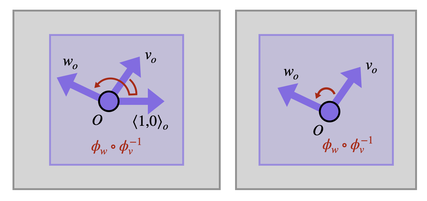
As a first example, suppose you wanted to show there is a rotation about \(O\) that takes some unit vector \(v\in T_{O}\EE^2\) to another unit vector \(w\in T_{O}\EE^2\). So far we only have one theorem about rotations - Theorem 11.4, which tells us that we can find one taking \(\langle 1,0\rangle_0\) to any vector. We will need to create two of these, and combine them via composition and inversion:
Proposition 11.1 For any two unit vectors \(v,w\in T_{O}\EE^2\), there is a Euclidean isometry which fixes \(O\) and sends \(v\) to \(w\).
Proof. Let \(\phi_v\) be a rotation taking \(\langle 1,0\rangle\) to \(v\), and \(\phi_w\) be an rotation taking \(\langle 1,0\rangle\) to \(w\): both of these are linear, and exist by Theorem 11.4. Now, consider the inverse function \(\phi_v^{-1}\). This is an isometry (by Exercise 11.4) which undoes the action of \(\phi_v\), so it fixes \(O\) and takes \(v\) to \(\langle 1,0\rangle\).

Now consider the composition \(\phi_w\circ\phi_v^{-1}\). This is a composition of isometries, and hence an isometry (Exercise 20). It fixes \(O\) since \(\phi_v^{-1}\) does and \(\phi_w\) does, so all we need to see is that it takes \(v\) to \(w\). So, just follow the vector \(v\)! We first feed it into \(\phi_v^{-1}\), which takes it to \(\langle 1,0\rangle\), and then we feed the result into \(\phi_w\), which takes \(\langle 1,0\rangle\) to \(w\)!
If you wanted to write this in symbols instead of pictures or words, it looks like this:
\[\begin{align*} D(\phi_w\circ\phi_v^{-1})_{O}(v)&=(D\phi_w)_{O}(D\phi_v^{-1})_{O}(v)\\ &=(D\phi_w)_{O}\left(\langle 1,0\rangle\right)\\ &= w \end{align*}\]
Next, we will look at trying to build an isometry that rotates around an arbitrary point \(p\) in the plane. We already found the isometries that rotate around \(0\): they are the nice linear maps of Theorem 11.4. But tracking down isometries that rotate around other points of the plane sounds more difficult. First of all - they cannot be linear maps! A linear map fixes the point \(O\), but a rotation about the point \(p\) fixes….\(p\)! However, combining a translation taking \(p\) to zero with a rotation about zero in the right way, we can succeed!
Theorem 11.5 Let \(p\) be a point in the Euclidean plane and \(v=\langle v_1,v_2\rangle\) a tangent vector based at \(p\). Then there is an isometry of \(\EE^2\) which fixes \(p\), and takes \(\langle 1,0\rangle\) to \(v\).
Proof. Let \(T\) be the translation \(T(q)=q+p\): this is an isometry by Theorem 11.3, and it takes \(O\) to \(p\). Also, let \(R\) be the rotation about \(O\) which takes the vector \(\langle 1,0\rangle\) based at \(O\) to the vector \(v_0=\langle v_1,v_2\rangle\) based at \(O.\) (Recall \(v_o\) means a vector with the same coordinates as \(v=v_p\in T_p\EE^2\), but based at \(0\) instead of \(p\).

From these, we construct the map \(\phi = T\circ R\circ T^{-1}\). This is an isometry because its a composition of isometries and their inverses (Exercise 20,Exercise 11.4), so we just need to check that it does what is claimed.
This fixes the point \(p\): since \(T\) takes \(O\) to \(p\), its inverse takes \(p\) to \(O\). Then \(R\) fixes \(O\), and finally, \(T\) takes \(O\) back to \(p\):
\[\begin{align*} \phi(p)&= TRT^{-1}(p)\\ &= TR(O)\\ &= T(O)\\ &= p \end{align*}\]
Next, we nee to check it does what we claim to the tangent vectors. To do so, we need to take the derivative of \(\phi\) at \(p\), and see that it takes \(\langle 1,0\rangle_p\) to \(v_p\). In symbols, we want to show \(D\phi_p(\langle 1,0\rangle_p)=v_p\).

We know by the proof of Theorem 11.3 that the derivative of \(T\) is the identity matrix. Thus, the derivative of \(T^{-1}\) is also the identity matrix (we differentiate an inverse by using the inverse of the derivative matrix, by Theorem 8.1). So applying \(DT^{-1}\) at \(p\) to \(\langle 1,0\rangle_p\) leaves it unchanged, except it moves the basepoint to \(O\) (since \(T^{-1}(p)=O\)).
Next, we apply \(R\). This fixes \(O\), and by Theorem 11.4 we know \(DR_o\) takes \(\langle 1,0\rangle_o\) to \(v_o\). Finally, we apply \(T\): since its derivative is the identity matrix it does not affect the coordinates of any vector just the basepoint, so it takes \(v_o\) to \(v_p\).
In symbols:
\[\begin{align*} D\phi_p(\langle 1,0\rangle_o)&=D(TRT^{-1})_p(\langle 1,0\rangle_o)\\ &= DT_o DR_o DT^{-1}_p (\langle 1,0\rangle_p)\\ &= DT_oDR_o(\langle 1,0\rangle_o)\\ &=DT_o(v_o)\\ &= v_p \end{align*}\]
Exercise 11.5 Can you modify the argument of Theorem 11.5 above to prove that in fact for any point \(p\) and any two unit tangent vectors \(v_p\), \(w_p\) in \(T_p\EE^2\), there is an isometry which fixes \(p\) and takes \(v_p\) to \(w_p\)?
Hint: look at the proof of Proposition 11.1 for inspiration.
This operation - move, then do your next trick, then undo the original movement is an extremely common manuever in mathematics to build new things from known things. Its essential not only in geometry, but also at the heart of abstract algebra and other fields, and is called conjugation.
Definition 11.3 (Conjugation) If \(a\) and \(b\) are two mathematical objects that can be multiplied or composed, then the object \[bab^{-1}\] is called the conjugate of \(a\) by \(b\).
Often, we will interpret this as doing the action determined by \(a\), at the location determined by \(b\). Thus we can describe the previous theorem much more succinctly with our new terminology: to rotate about the point \(p\), we conjugate a rotation about \(0\) by a translation from \(0\) to \(p\). Or - we perform a rotation at the location we translate to.
11.3 Homogenity and Isotropy
The fundamental property of Euclidean geometry that allowed the greeks and ancients to make so much progress was the incredible amount of symmetry that the plane has. It doesn’t matter where you draw a triangle, a circle or another figure: all locations of the plane look and act the same. This concept that space looks the same at every point and also behaves the same in every direction is fundamental to modern geometry
Definition 11.4 (Homogeneous Space) A space is homogeneous if for every pair of points in the space, there is an isometry taking one to the other.
Definition 11.5 (Isotropic Space) A space is isotropic if for any point \(p\) and any two directions leaving \(p\), there is a rotation of the space taking one direction to the other.
The existence of translations shows us that the Euclidean plane is homogeneous, while the ability to rotate about any point shows us that it is isotropic.
Theorem 11.6 (Euclidean space is Homogeneous and Isotropic)
In practice, we will use the homogenity and isotropy of Euclidean space to simplify a lot of arguments. Once we prove something is true at one location (like the origin, where calculation is simple) we will immediately be able to deduce that the analogous theorem is true at all other points of the plane! To make such arguments, its useful to repackage homogenity and isotropy into a useful tool.
Proposition 11.2 (Moving from \(p\) to \(q\).) Given any two pairs \(p,v_p\) and \(q,w_q\) of points \(p,q\) in Euclidean space and unit tangent vectors \(v_p\in T_p\EE^2\), \(w_q\in T_q \EE^2\) based at them, there exists an isometry taking \(v_p\) to \(w_q\).
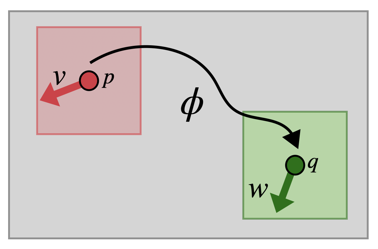
Exercise 11.6 Prove Proposition 11.2 above.
Hint: use Theorem 11.3 to construct isometries taking \(O\) to both \(p\) and \(q\), and Proposition 11.1 to build the right sort of rotation around \(O\) that you need. Compose these (or their inverses) to get a map taking \(v_p\) to \(v_o\), then to \(w_o\), and finally to \(w_p\).
11.4 Similarities
Isometries - maps that preserve all infinitesimal lengths - are very special among the collection of all possible maps of the plane. Most mappings \(F\colon\EE^2\to\EE^2\) don’t do anything understandable to lengths!
However, there is one important intermediate ground of maps: they don’t preserve distances - but they don’t change them arbitrarily either. We will call a map a similarity if it scales all infinitesimal lengths by the same factor:
Definition 11.6 An map \(\sigma\colon \EE^2\to\EE^2\) is called a similarity if there is a positive real number \(k\) such that \[\|D\sigma_p(v)\|=k\|v\|\] for all tangent vectors \(v\). This constant \(k\) is called the scaling factor or dilation of the map \(\sigma\).

Perhaps the simplest similarities of the plane are given by vector scalar multiplication: just take the map \(\sigma(x,y)=(kx,ky)\).
Example 11.3 The map \(\sigma(x,y)=(2x,2y)\) is a similarity with scaling factor \(2\). Computing its derivative we see \[D\sigma = \pmat{2&0\\0&2}\] and so for any point \(p\) and any vector \(v\in T_p\) applying \(D\sigma_p\) just multiplies all its coordinates by \(2\). Thus if \(v=\langle v_1,v_2\rangle_p\), \[\|D\sigma_p(v)\|=\|\langle 2v_1,2v_2\rangle\|=2\|\langle v_1,v_2\rangle\|=2\|v\|\] Since this is the same constant for every vector \(v\), this implies that \(\sigma\) is a similarity!K
Because similarities do exactly the same thing to every tangent vector in the plane, we can compute exactly how they scale the lengths of curves.
Proposition 11.3 (Similarities Scale Lengths) Let \(\gamma\colon[a,b]\to\EE^2\) be a curve, and \(\sigma\) a similarity with scaling factor \(k\). Then \[\len(\sigma\circ\gamma)=k\len(\gamma)\]
Proof. We compute the length of \(\sigma\circ\gamma\) via an integral: \[\begin{align*} \len(\sigma\circ\gamma)&=\int_a^b \|(\sigma\circ\gamma)^\prime(t)\|dt\\ &=\int_a^b\|D\sigma_{\gamma(t)}\gamma^\prime(t)\|dt\\ &=\int_a^b k\|\gamma^\prime(t)\| dt\\ &=k\int_a^b\|\gamma^\prime(t)\|dt\\ &=k\len(\gamma) \end{align*}\] Where in the middle we used the fact that \(\sigma\) was a similarity so \(\|D\sigma(v)\|=k\|v\|\) for any vector \(v\).

Just like for isometries, we have as a theorem of calculus that this condition actually implies that our map is invertible! We will not prove this theorem here, and if you like you can instead treat this as an extra condition we require of a function to be a similarity.
Theorem 11.7 (Every Similarity is Invertible)
For isometries, you proved the inverse of an isometry is an isometry (Exercise 11.4) by showing that if \(\phi\) didn’t change the length of any vectors, than neither could \(\phi^{-1}\). Here we investigate the analogous question for similarities.
Proposition 11.4 If \(\sigma\) is a similarity with scaling factor \(k\), then \(\sigma^{-1}\) is also a similarity, this time with scaling factor \(1/k\).
Proof. Let \(\sigma\) be such a similarity, and \(\sigma^{-1}\) be its inverse. Then by definition we know their composition is the identity function $ \[\sigma\circ\sigma^{-1} = \mathrm{id}\] The identity function \((x,y)\mapsto (x,y)\) has the identity matrix as its derivative. On the other side, we can use the multivariable chain rule to get
\[D(\sigma\sigma^{-1})_p=D\sigma{\sigma^{-1}(p)}D\sigma^{-1}_p = I\]
Now start with any vector \(v\) based at a point \(p\). We first feed this vector into \(D\sigma^{-1}_p\), which returns a new vector - let’s call it \(w\). We don’t know anything about \(w\) at the moment, but we do know that when we feed it into \(D\sigma\), its length will multiply by \(k\), since \(\sigma\) is a similarity. But we know more than this! The end result must be literally the vector \(v\): since we started with \(v\) and the composition of \(D\sigma\) with \(D\sigma^{-1}\) is the identity matrix.
Thus we know that whatever \(w\) is, when you multiply its length by \(k\) you get the length of \(v\), so \[k\|w\|=\|v\|\] But - remember \(w\) is just the vector \(D_p\sigma^{-1}(v)\): so we’ve found \[\|D\sigma^{-1}_p(v)\|=\frac{1}{k}\|v\|\] And this holds for all vectors \(v\) - so the inverse is indeed a similarity, and the scaling constant is \(1/k\).
More generally, we can use the same sort of reasoning to understand compositions of any similarities.
Exercise 11.7 Prove that the composition of a similarity and isometry is another similarity, with the same scaling factor.
Exercise 11.8 If \(\sigma\) and \(\psi\) are two similarities with scaling constants \(c\) and \(k\) respectively, the composition \(\sigma\circ\psi\) is also a similarity, with scaling constant \(ck\).
From this, we can build many more similarities from the simple ones we know.
Exercise 11.9 The similarities \((x,y)\mapsto (kx,ky)\) fix \(O\) in the plane: can you use translations to build a similarity with scaling constant \(k\) which instead fixes the point \(p=(a,b)\)?