$$ \newcommand{\RR}{\mathbb{R}} \newcommand{\QQ}{\mathbb{Q}} \newcommand{\CC}{\mathbb{C}} \newcommand{\NN}{\mathbb{N}} \newcommand{\ZZ}{\mathbb{Z}} \newcommand{\EE}{\mathbb{E}} \newcommand{\HH}{\mathbb{H}} \renewcommand{\SS}{\mathbb{S}} \newcommand{\DD}{\mathbb{D}} \newcommand{\pp}{^{\prime\prime}} \newcommand{\p}{^\prime} \newcommand{\proj}{\operatorname{proj}} \newcommand{\area}{\operatorname{area}} \newcommand{\len}{\operatorname{length}} \newcommand{\acc}{\operatorname{acc}} \newcommand{\ang}{\sphericalangle} \newcommand{\map}{\mathrm{map}} \newcommand{\SO}{\operatorname{SO}} \newcommand{\dist}{\operatorname{dist}} \newcommand{\length}{\operatorname{length}} \newcommand{\uppersum}[1]{{\textstyle\sum^+_{#1}}} \newcommand{\lowersum}[1]{{\textstyle\sum^-_{#1}}} \newcommand{\upperint}[1]{{\textstyle\smallint^+_{#1}}} \newcommand{\lowerint}[1]{{\textstyle\smallint^-_{#1}}} \newcommand{\rsum}[1]{{\textstyle\sum_{#1}}} \newcommand{\partitions}[1]{\mathcal{P}_{#1}} \newcommand{\erf}{\operatorname{erf}} \newcommand{\pmat}[1]{\begin{pmatrix}#1\end{pmatrix}} \newcommand{\smat}[1]{\left(\begin{smallmatrix}#1\end{smallmatrix}\right)} $$

6 Fundamental Strategy

Calculus is the story of humanity’s quest to understand infinity: dealing with the infinitely small (differentiation), infinitely large (convergence), and processes that occur infinitely often (sequences, and infinite series). Out of this philosophical quandries grew an extremely useful set of mathematical tools that radically changed our world.

No longer were we constrained by the straight line geometry of the Greeks, or even the algebra of polynomials from the Middle East. The new mathematical tools provided a means of calculating - or a calculus with arbitrary curves.

The Fundamental Strategy of Calculus Upon zooming in far enough, functions appear linear. At this level of zoom, you can replace difficult (nonlinear) problems with simple (linear) ones

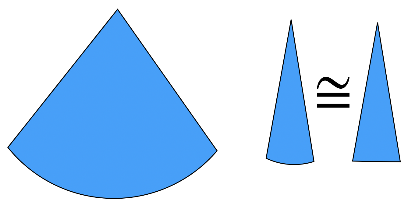
This was Archimedes’ fundamental insight. In trying to compute the area of a circle, he divided it into small circular wedges. Of course, it was no easier to calculate the area of a wedge than it was to calculate the area of the circle as a whole - as each wedge still had a curved (nonlinear) side. But - as the number of wedges grew - each wedge shrank, and allowed us to zoom in on a smaller and smaller piece of the curve. The farther we zoom, the closer this small curved arc is approximated by a straight line - making our problem into a linear one: we replace the area of a curved sector with the area of a triangle!

Large circular sectors are not well approximated by triangles But *small* circular sectors only have a tiny piece of circular arc. Tiny arcs are approximately linear, so small sectors *are* well approximated by triangles.

This insight was discovered time and again over the following twenty centuries, by mathematicians the world over. As this is a geometry course - and not one on the history of calculus - we will not have the time to treat many of these amazing insights with the respect and awe they deserve. (Though, for those interested in such matters - consider taking Real Analysis with me in the spring!).

6.1 Infinitesimal Space

In the original, pre-rigorous formulations of calculus, mathematicians had the correct picture in their minds - that if you zoom in far enough on any smooth graph, it should look linear. But they had difficulty putting this intuition on a firm mathematical footing. Of course, at any finite level of zoom the curve is not linear, but still curves very slightly! It’s only in the limit of infinite zoom that this approximation becomes exact.

But at the level of infinite zoom, what is the resulting line made out of? It can’t be made out of regular points $(x,y)$ on the plane: as these points are what makes up the curve. It must instead be made out of some new, infinitesimally small numbers. The intuition was that infinitely near every number $x$ on the line, there were also infinitesimal numbers nearer to $x$ than any other other “normal” (finite) real number. And infinitesimally near any point $p$ in the plane, there were infinitesimally small points.

But immediately from this idea sprung forth many questions: how many of these infinitely small numbers must there be? If $\epsilon$ is one of these infinitesimals near $x$, then what about $2\epsilon$? That must still be infinitesimally near to $x$, as $\epsilon$ is so so so small! Similarly, $k\epsilon$ must be infinitesimally near $x$ for any $k$: there’s an entire number line of infinitesimal numbers near every real number!

What about in the plane? If $v$ and $w$ are two points infinitesimally close to $p$, then what about $v+w$, or $kv+cw$ for scalars $k,c$? These must also be infinitesimally near $p$: so it appears there is an entire plane of infinitesimal points that must be near every finite point!

This mental picture seemed to make perfect sense, but there were some deep questions. What are the rules of arithmetic for infinitesimally small numbers? Using arithmetic for just infinitesimal numbers alone, or just finite (normal) numbers alone posed no trouble, but strange things happened if you tried to combine them. If $\epsilon$ is infinitely close to zero, what is the number $1/\epsilon$? It must be bigger than all normal numbers: so, is it infinity? But then what is $2/\epsilon$? Another infinity larger than the first? Luckily, we don’t have to worry about these questions, as during the development of Real Analysis mathematicians proved an important theorem:

Theorem 6.1 The real line does not contain any infinitesimal numbers.

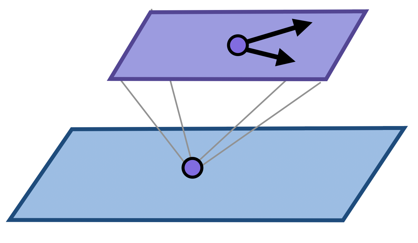
This tells us as geometers that we should not be trying to combine the arithmetic of finite and infinitesimal numbers, and should instead keep them separate! This in fact makes things easier: at each point of the plane we have a plane of infinitesimal numbers, but different infinitesimal planes do not mix together, or with the points of the space. Because we often use these infinitesimal numbers to describe tangents to curves, the modern terminology for these infinitely zoomed in spaces are tangent spaces

Definition 6.1 (Tangent Space to the Line) To every point $x\in\RR$, there is attached a separate real line of infinitesimal numbers, denoted $T_x\RR$ and called the *tangent space to $\RR$ at $x$. Inside a fixed tangent space we can write down linear equations, but points of $T_x\RR$ cannot be combined with points of $\RR$ itself, or $T_y\RR$ for any other point $y$.

There is a *separate* line of infinitesimal numbers attached to every single point.

Definition 6.2 (Tangent Space to the Plane) To every point $p\in\RR^2$, there is attached a separate plane of infinitesimal vectors, denoted $T_p\RR^2$ and called the *tangent space to $\RR^2$ at $p$. Inside a fixed tangent space the rules of linear algebra apply, but points of $T_p\RR^2$ cannot be combined with points of $\RR^2$ itself, or $T_q\RR$ for any other point $q$.

Remark 6.1. “Nice enough” here means that when you zoom in, linear algebra begins to apply. The collection of spaces for which this is possible are called manifolds.

These definitions look very similar, and invite an immediate generalization. If $X$ is any nice enough space, we can define the tangent space at every point as a vector space attached to that point, with the same dimension as $X$. We will make use of this more and more as the book progresses.

To keep things straight, its useful to have some notation for tangent vectors, that will help us remember where they are based at.

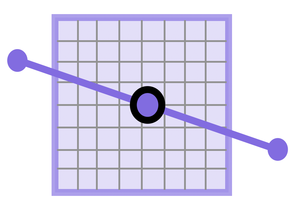
Definition 6.3 Let $X$ be a space (the line, the plane, etc) and let $p$ be a point of $X$. Then we denote the tangent space at $p$ as $T_pX$, and when we need to be extra-precise, we put $p$ a subscript even on individual vectors, to show they live in $T_pX$. For example

\[v_p = \langle 1,2\rangle_p =\pmat{1\\ 2}_p\]

A warning - if you don’t keep careful track of where a vector is based, its easy to get confused! The vector $\langle 1,1\rangle$ may represent an infinitesimal vector based at $p=(1,1)$ or an infinitesimal vector based at $q=(0,1)$: but these two infinitesimal vectors are different!

Tangent vectors at different points truly live in different spaces, even if they have the *same description with coordinates*. It’s always important to keep track of where a vector is based.

This will feel much more natural once we start actually doing calculus in this way.

6.2 Implementation

In broad strokes, modern applications of calculus follow closely Archimedes template. Given a difficult, nonlinear problem, the first step is to zoom in: to look infinitesimally in the tangent space of every point, where the problem simplifies and becomes linear.

Zooming in to each tangent space replaces the original function with a *linear function*.

While zoomed in, we work infinitesimally and simplify the problem as much as possible, taking advantage of the linear mathematics we now have to work with.

Working infinitesimally often involves linear equations.

Once we have succeeded at this, we zoom out: piecing back together the infinitesimal linear information from all the relevant points into finite information answering the original question.

Zooming out: combining infinitely many linear problems to solve one nonlinear problem.

These steps may look different from problem to problem, but the overall strategy remains unchanged. Most of the time the zoom in step involves some form of differentiation, or tangent line approximation, but the zoom out step can be more varied. The most common means of zooming out is integration combining infinitesimal information from an infinite continnuum of points. But infinite summation is also a means of zooming out - combining together an infinite sequence of infinitesimal terms. And sometimes, zooming out requires no extra work at all: if we can solve the problem completely at the infinitesimal level, our zoom out is only to come back up to reality and report the answer.

Below are several familiar examples of the fundamental strategy in action, so you can see the variety of methods fitting this general framework.

Example 6.1 (Area Under a Curve) Starting with a continuous function on an interval $[a,b]$ in the real line, the goal is to find the area between the graph of $f$ and the $x-$axis, from $x=a$ to $x=b$:

Zoom In: If we look infinitesimally near a single point $x$, we can approximate $f$ as constant (even better than linear!).

Work Infinitesimally: Thus the infinitesimal area is given by an infinitesimal rectangle as the top side is no longer curved.

Zoom Out: To get the total area, we need to combine together (sum up) the areas of these infinitesimal rectangles. At any finite level of zoom this would be a (Riemann) sum, but at the infinite level of zoom of calculus, this becomes an integral!

\[\mathrm{Area}=\int_a^b f(x)dx\]

Example 6.2 (Archimedes’ Parabola) To find the area under a parabolic segment, Archimedes followed a similar approach, though without the modern theory of integration. This makes the application of the fundamental strategy even more clear.

Zoom In: Fill the parabolic segment with more and more triangles. As the triangles get smaller, they zoom in more and more on smaller segments of the parabola, which are better and better approximated by the straight edges of the triangles.

Work Infinitesimally: The area of each triangle is easy to calculate, and the relationships between the areas of different triangles (for instance, those in level $n$ vs those in level $n+1$) is deducible using Euclidean geometry. It turns out, the areas of the triangles follow a pattern - at each level the new contribution is $1/4$ the area of the previous.

Zoom Out: To find the area of the entire parabola, we must sum the areas accumulated at every level. Its no longer relevant where these numbers came from as we know the pattern: each number in the list is $1/4^{th}$ the previous. Its a geometric series! So zooming out requires us only to sum this series - the sum gives the total area.

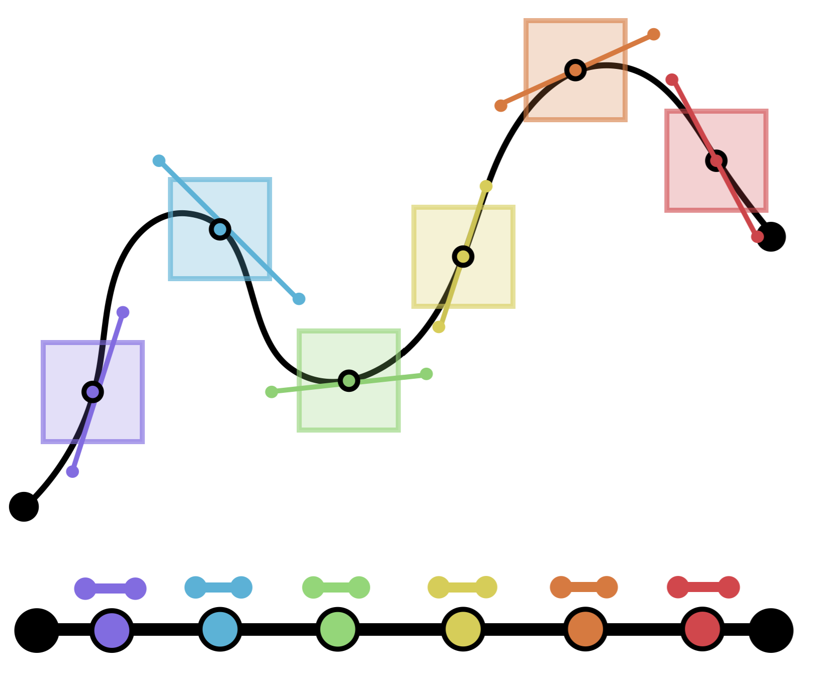
Example 6.3 (Computing Function Values) Consider the problem of evaluating a function line $\sin(x)$: what is the value of $\sin(0.23)$? Unlike polynomials the sine doesn’t seem to have a nice formula that we can just plug $0.23$ into…so, we use calculus to find one!

Zoom In: Some values of $\sin(x)$ we do know how to calculate well: the simple multiples of $\pi$ that appear on the unit circle. So, we will zoom in on one of these: here choosing $x=0$ (as its close to $0.23$). At this point, we cannot see anything about $\sin(x)$ except its value, and the value of its derivatives at $0$.

Work Infinitesimally: Differentiating $\sin$ repeatedly we see a pattern: its derivative cycles through the following list: $\sin, \cos, -\sin,-\cos$ and then repeats. We know how to evaluate both $\sin$ and $\cos$ at $x=0$, so we can evaluate all the derivatives: \[f(0)=0,\; f^\prime(0)=1,\; f^{\prime\prime}(0)=0,\; f^{\prime\prime\prime}(0)=-1,\; f^{\prime\prime\prime\prime}(0)=0\cdots\]

Zoom Out: Now that we know the infinitesimal pattern, we must assemble all this information into a function. Its easy to write down a linear function with $f(0)=0$, $f^\prime(0)=1$, jsut take $f(x)=x$. To also get $f^{\prime\prime}(0)=0$ and $f^{\prime\prime\prime}(0)=-1$ we need a cubic function: $f(x)=x-\frac{1}{6}x^3$. And to get all the derivatives right we need an infinite series!

\[\sin(x)=x-\frac{1}{3!}x^3+\frac{1}{5!}x^5-\frac{1}{7!}x^7+\cdots\]

Summing this series at any point $x$ gives the value of $\sin$ at that point - even though we only used the infinitesimal information at $x=0$ to derive it! With this formula, its no trouble to evaluate $\sin(0.23)$, or any other value.

Example 6.4 (Maximizing a Function) Given a smoothly varying function $f(x)$ on an interval $[a,b]$, a difficult problem is to find the point $x_0$ at which $f(x)$ is largest.

Zoom In: Our main insight is that when a function has reached its maximum value, it changes from increasing (before the peak) to decreasing (after the peak). Zooming in at some point $x$ inside the interval $(a,b)$, the rate of change of $f$ at that point is captured by the derivative. So we just need to study the derivative.

Work Infinitesimally: If a function is increasing the derivative is positive, and when its decreasing it’s negative. So, when it switches from increasing to decreasing, we must have $f^\prime(x)=0$. This has replaced a calculus problem (maximization) with an algebra problem (solving for the zero of a function).

Zoom Out: To zoom back out, we need to consider the entire interval and make sure we have found the answer. The calculus procedure above let us find all the points where $f^\prime(x)=0$ inside the interval - these are potential places for the maximum to occur. The other potential places are at teh endpoints of the interval. So, we need to compare the value of $f$ all these points, and report the largest value we found.

In this Part of the book, we will do a deep dive into these three components of the fundamental strategy, so that we can utilize this powerful tool in the rest of our geometric investigations. First, we will learn about working infinitesimally - that is, what linear functions look like in one and two dimensions. Then we will learn how to zoom in - starting with a nonlinear function and differentiating it to get something linear. And finally, we will review methods of zooming out: integration and power series.