$$ \newcommand{\RR}{\mathbb{R}} \newcommand{\QQ}{\mathbb{Q}} \newcommand{\CC}{\mathbb{C}} \newcommand{\NN}{\mathbb{N}} \newcommand{\ZZ}{\mathbb{Z}} \newcommand{\EE}{\mathbb{E}} \newcommand{\HH}{\mathbb{H}} \renewcommand{\SS}{\mathbb{S}} \newcommand{\DD}{\mathbb{D}} \newcommand{\pp}{^{\prime\prime}} \newcommand{\p}{^\prime} \newcommand{\proj}{\operatorname{proj}} \newcommand{\area}{\operatorname{area}} \newcommand{\len}{\operatorname{length}} \newcommand{\acc}{\operatorname{acc}} \newcommand{\ang}{\sphericalangle} \newcommand{\map}{\mathrm{map}} \newcommand{\SO}{\operatorname{SO}} \newcommand{\dist}{\operatorname{dist}} \newcommand{\length}{\operatorname{length}} \newcommand{\uppersum}[1]{{\textstyle\sum^+_{#1}}} \newcommand{\lowersum}[1]{{\textstyle\sum^-_{#1}}} \newcommand{\upperint}[1]{{\textstyle\smallint^+_{#1}}} \newcommand{\lowerint}[1]{{\textstyle\smallint^-_{#1}}} \newcommand{\rsum}[1]{{\textstyle\sum_{#1}}} \newcommand{\partitions}[1]{\mathcal{P}_{#1}} \newcommand{\erf}{\operatorname{erf}} \newcommand{\pmat}[1]{\begin{pmatrix}#1\end{pmatrix}} \newcommand{\smat}[1]{\left(\begin{smallmatrix}#1\end{smallmatrix}\right)} $$

10 Foundations

Definition 10.1 (Points of $\EE^2$) The points of the Euclidean plane are pairs $p=(x,y)$ of real numbers: that is \[\mathbb{E}^2=\{(x,y)\mid x,y\in\RR\}\cong\RR^2\]

The Plane is built out of the points of $\RR^2$, together with a tangent space at each point.

We use the notation $\EE^2$ for the geometry even though the underlying point set is just the plane $\RR^2$ This is because ordered pairs of real numbers can represent many different things (see ?sec-maps) and we wish to make it clear here that right now we mean their original usage, to describe the geometry of Euclid.

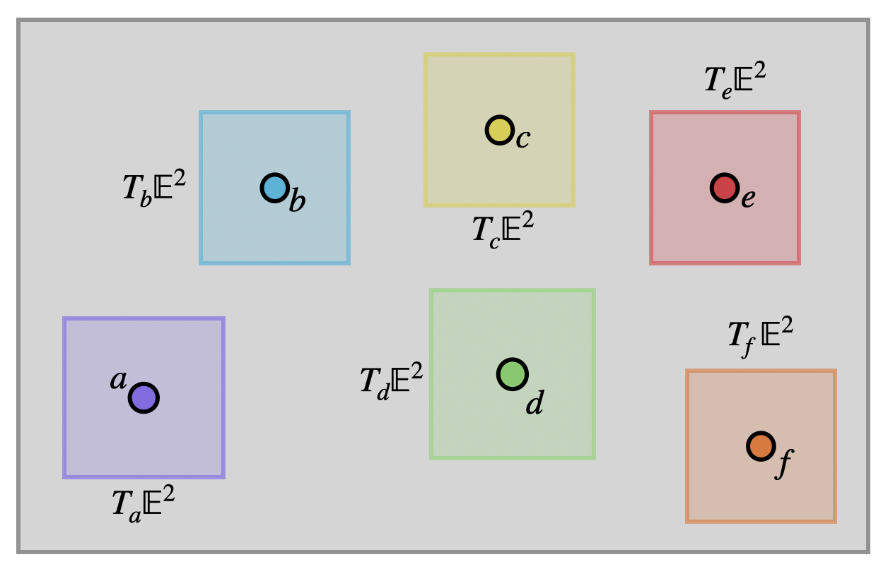
Definition 10.2 (Vectors of $\EE^2$) At each point $p$ of the Euclidean plane, the set of tangent vectors is another copy of $\RR^2$.
\[T_p\EE^2=\{(v_1,v_2)\mid v_i\in\RR\}\cong\RR^2\]

Vectors are just pairs of real numbers as we are used to, but we do need to be careful about keeping track of where they are based. Hence, we will often write a subscript on a vector to denote where it lives: $\langle 1,2\rangle_{(1,5)}$ is the vector $\langle 1,2\rangle$ based at $(1,5)\in\EE^2$, whereas $\langle 1,2\rangle_{(-2,3)}$ is the vector with teh same coordinates, but based at $(-2,3)$.

The origin is the point with coordinates $(0,0)$ in the plane. Because these zeroes will make some calculations easier, we will often find ourselves doing things at the origin, and so its useful to have a shorthand notation. We will write $O=(0,0)$ for this point, and denote vectors based at $O$ with the subscript $v_o$, consistent with the above.

Now we have a precise definition of what the Euclidean plane is made out of (points) and its infinitesimal pieces ( vectors), so we can precisely define things like curves and their tangents.

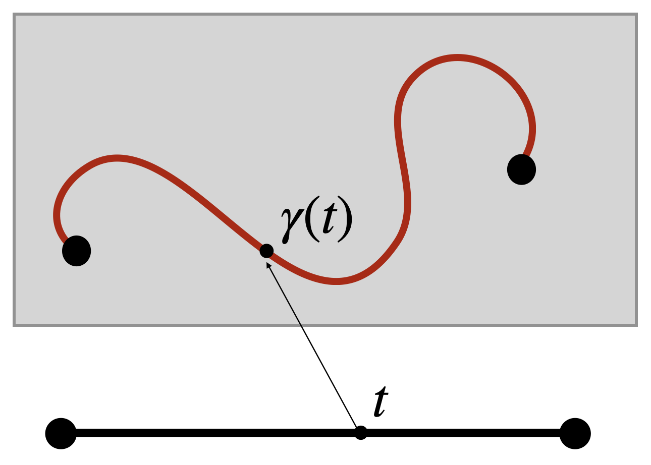
A curve is a function from an interval in $\mathbb{R}$ into the Plane.

Definition 10.3 (Curves) A curve in the Euclidean plane is a function $\gamma\colon I\to \EE^2$ for $I$ an interval in the real line (or possibly all of $\RR$). The tangent to $\gamma(t)=(x(t),y(t))$ at time $t_0$ is its coordinate-wise derivative \[\gamma^\prime(t_0)=\langle x^\prime(t_0),y^\prime(t_0)\rangle \in T_{\gamma(t_0)}\EE^2\]

A curve is regular if its derivative is never equal to the zero vector for ant $t\in I$.

But to make real progress, we need the tools to be able to measure length.

10.1 Length of Curves

Our new formulation of geometry puts all curves on an equal footing - an allows us to measure their lengths using the ideas of calculus. This was the dream of Archimedes, realized only nearly two millennia after his death.

Idea: infinitesimally, geometry looks like what was studied by the greeks, as if you zoom in on any curve it appears as a line. To impose this fact on our new geometry we will measure infinitesimal distances via the pythagorean theorem. This will be our only geometric axiom - from this alone (together with the tools of calculus) we will rebuild all of geometry.

The fundamental axiom of the plane - the Pythagorean Theorem is true infinitesimally, in each tangent space.

Definition 10.4 (Infinitesimal Length in $\EE^2$) If $v$ is a tangent vector based at $p\in\EE^2$ then its infinitesimal length is given by the pythagorean theorem on the tangent space $T_p\EE^2$. \[\|v\|=\sqrt{v_1^2+v_2^2}\]

To measure a curve we take inspiration from Archimedes’ measurement of the circle and approximate it with small line segments. A curve is called rectifiable if these approximate lengths converge as their number tends to infinity. It’s a consequence of calculus that regular curves are rectifiable.

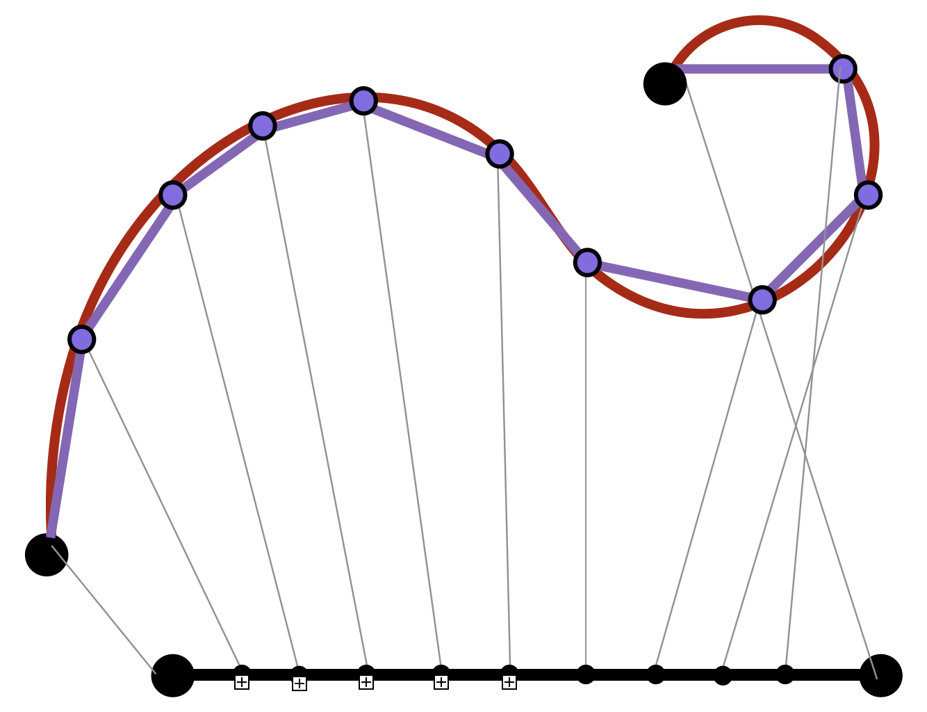
The spirit of Archimedes: we can figure out how to define the length of a curve by thinking about approximations to it.

Then we define the length of real curves by zooming out (integrating) their zoomed-in (differential) lengths. Unlike in Euclid’s formulation, now all curves are on an equal footing: all lengths are determined by infinitesimal integration!

Definition 10.5 (Length in $\EE^2$) If $\gamma$ is a curve which is differentiable, then we can measure the length of $\gamma(t)$ from $t=a$ to $t=b$ by integrating the infinitesimal lengths of its tangent vectors: \[\len(\gamma)=\int_a^b \|\gamma^\prime(t)\|dt\]

The derivative $\gamma^\prime(t)$ is a linear map taking an infinitesimal vector at $t$ to an infinitesimal piece of arc at $\gamma(t)$. Integrating the lengths of these infinitesimal vectors is how we *define* the length of a curve.

Its helpful to write this definition out in full: if $\gamma(t)=(x(t),y(t))$ then $\gamma^\prime(t)=\langle x^\prime(t),y^\prime(t)\rangle$ and so $\|\gamma^\prime(t)\|=\sqrt{x^\prime(t)^2+y^\prime(t)^2}$. Thus

\[\len(\gamma)=\int_a^b\sqrt{x^\prime(t)^2+y^\prime(t)^2}dt\]

Such integrals can be difficult to do in practice because of that nasty square root that shows up in their definition. And when they are possible, these often need several calculus tricks to succeed:

Exercise 10.1 (The Length of a Parabola) Find the length of the parabola $y=x^2$ between from $x=0$ to $x=a$, following the steps below.

Parameterize the curve as $c(t)=(t,t^2)$, show the arclength integral is $L(a)=\int_{[0,a]}\sqrt{1+4t^2}$
Perform the trigonometric substitution $x=\frac{1}{2}\tan\theta$ to convert this to some multiple of the integral of $\sec^3(\theta)$.
Let $I=\int\sec^3(\theta)d\theta$ and do integration by parts with $u=\sec\theta$ and $dv=\sec^2\theta$.
After parts, use the trigonometric identity $\tan^2\theta=\sec^2\theta-1$ in the resulting integral to get another copy of $I=\int\sec^3\theta d\theta$ to appear.
Get both copies of $I$ to the same side of the equation and solve for it! To check your work at this stage, you should have found that \[\int\sec^3\theta d\theta = \frac{1}{2}\sec\theta\tan\theta+\frac{1}{2}\ln\left|\sec\theta+\tan\theta\right|\]
Relate this back to your original integral, and undo the substitution $x=\frac{1}{2}\tan\theta$: can you use some trigonometry to figure out what $\sec\theta$ is?
Finally, you have the antiderivative in terms of $x$! Now evaluate from $0$ to $a$.

Our main use isn’t to compute the lengths of a bunch of random curves. Instead, its more theoretical - the integral gives a precise definition for the length of any differentiable curve, and a simple definition at that! This will be extremely useful in building geometry back from our small foundations.

10.1.1 Parameterization Invariance

All seems well and good with this definition, but the mathematician in us should be a little worried: we defined the length of a curve in terms of a parameterization, but the curve itself doesn’t care how we parameterize it!

To get a sense of this its easiest to look at an explicit example: below are four different curves which all trace out the same set of points in the plane: the segment of the $x$ axis between $0$ and $4$.

\[\alpha(t)=(t,0)\hspace{1cm}t\in[0,4]\] \[\beta(t)=(2t,0)\hspace{1cm}t\in[0,2]\] \[\gamma(t)=(t^2,0)\hspace{1cm}t\in[0,2]\]

Because these all describe the same set of points, we of course want them to have the same length! But our definition of the length function involves integrating infinitesimal arclengths (derivatives), and these curves don’t all have the same derivative! Thus, to really make sure our definition makes sense, we need to check that it doesn’t matter which parameterization we use, we will always get the same length.

Exercise 10.2 Check these three parameterizations of the segment of the $x$-axis from $0$ to $4$ all have the same length.

Two curves are said to have the same image if the set of points they trace out in the plane are the same. So, all three of the curves above have the same image, and the same length. This requires a bit more calculus to check in general, but remains true.

Two curves $\beta$ and $\gamma$ with the same image.

Theorem 10.1 (Length & Parameterization Invariance) If $\beta$ and $\gamma$ are two curves with the same image, then \[\len(\beta)=\len(\gamma)\]

Proof. Let $\beta(s)\colon [a,b]\to \EE^2$ and $\gamma(t)\colon [c,d]\to\EE^2$ be two curves with the same image. That means they trace out the same set of points in the plane, so for every value of the parameter $t$ for $\gamma$ there is some value of $s$ for $\beta$ where $\beta(s)=\gamma(t)$. Write $s(t)$ for the function that does this - chooses the matching $s$ parameter for each $t$.

The function $s(t)$ which takes the $t$ parameter for the curve $\gamma$, and returns the $s$ parameter for the curve $\beta$ which maps to the same point in $\EE^2$.

We can use this to wite the curve $\gamma$ *in terms of $\beta$, as $\gamma(t)=\beta(s(t))$. We now calculate the length of $\gamma$ using the definition:

\[\begin{align*}\len(\gamma)&=\int_{[c,d]}\|\gamma^\prime(t)\|dt\\ &= \int_{[c,d]}\|\beta(s(t))^\prime\|dt\\ &= \int_{[c,d]}\|\beta^\prime(s(t))s^\prime(t)\|dt \end{align*}\]

Where we used the chain rule in the last step to differentiate the composition. Now, $\beta^\prime$ is a vector, but $s(t)$ was a scalar function so $s^\prime(t)$ is a scalar, and we can pull it out of the norm, and do a $u$-substitution! Picking up from where we left off,

\[\begin{align*} &=\int_{[c,d]}\|\beta^\prime(s(t))\|s^\prime(t)dt\\ &=\int_{[s(c),s(d)]}\|\beta^\prime(s)\|ds\\ &=\int_{[a,b]}\|\beta^\prime(s)\|ds\\ &=\len(\beta) \end{align*}\]

:::{#rem-curves} T here are some things we need to be careful on here: the curves $\beta$ and $\gamma$ are regular - their derivatives are never zero - which implies that they trace the curve from start to finish without stopping or doubling back. This, together with the fact that the curves are traced in the same direction implies that $s^\prime(t)$ is always positive, which justifies the use of $u$-substitution. :::