18 Lines & Circles
Now that we’ve made it through the fundamentals of spherical geometry, we are ready to move on from the infinitesimal to the actual, finite geometric properties we are usually interested in.
In this section, again much of the details will be similar to what we have already seen in the Euclidean plane, and because of those similarities we will be able to make rather fast progress. However the actual statements we can prove will start to differ - signaling something is truly different about this geometry. We will take up the cause of this difference - curvature - in the following chapter.
18.1 Lines
In Euclidean geometry we considered several distinct definitions of the term line, and then proved that all three definitions pick out the same class of curves. This allowed us the freedom to freely switch between the three definitions,
- Length Minimizing
- Straightest
- Lines of Symmetry
when convenient. The same holds for the sphere: when we are seeking the fundamental curves of this geometry we can either look for length minimizers, or for curves that do not turn, or curves that are fixed by an isometry.
I will often call a curve satisfying any of these three equivalent properties a line, because these curves play the same role in the theory of the sphere that our original lines do in the plane. But theres a more ancient term which originated with the sphere, and is now commonly used for this generalization of line all across mathematics.
Remark 18.1. Careful readers will notice that here I am just claiming that all three definitions remain the same on the sphere, we have not yet proved it. We will prove it in time, but it will be best to wait until we have developed some more tools, so we can avoid difficult and unenlightening integrals.
Definition 18.1 (Geodesic) A geodesic on the sphere is a curve satisfying any of the three equivalent properties which defined lines in the plane.
The term geodesic is Greek, originally deriving from γεωδαισία, or division of earth, as a line across the surface of the earth divides it in two. This grew into geodesy or measurement of the earth in english, and then to geodesic in mathematics.
18.1.1 Curves Fixed by Isometries
Because we just spent all this effort dealing with isometries it will turn out to be easiest to discover which curves are lines using the lines of symmetry definition. Recall that we say a point \(p\) is fixed by an isometry \(\phi\) if \(\phi(p)=p\). Analogously, we say that an entire curve \(\gamma\) is fixed by \(\phi\) if for each value of \(t\), the point \(\gamma(t)\) is fixed by \(\phi\) - like the line a mirror sits on when it reflects the plane. What is the analog on \(\SS^2\)?
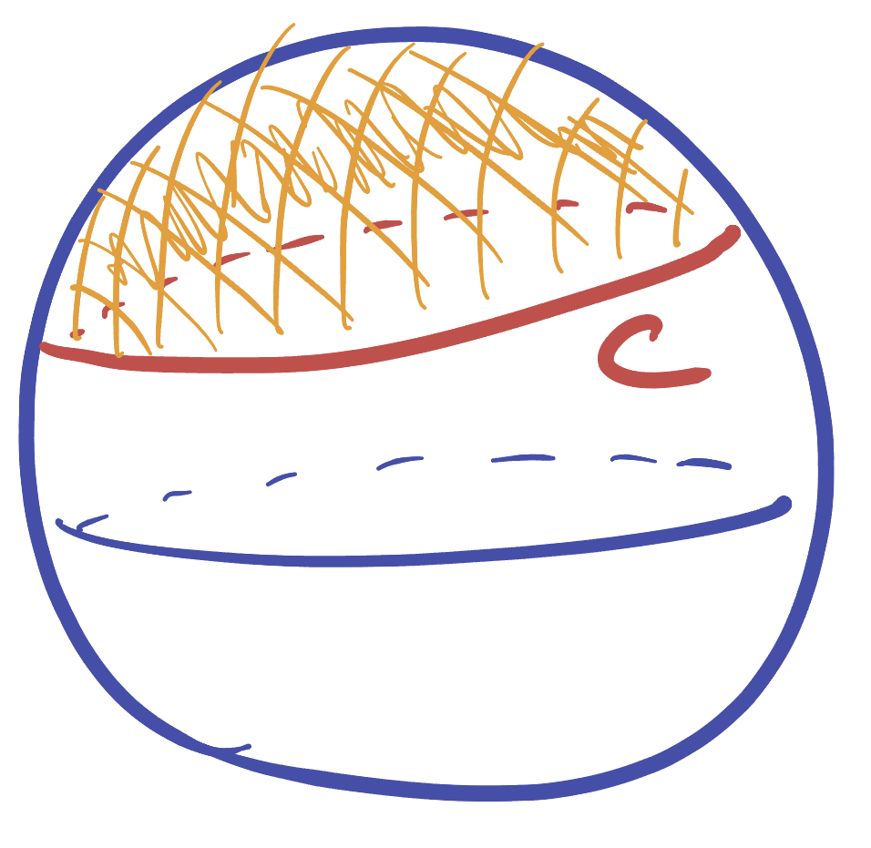
Example 18.1 The equator \((x,y,0)\) of the sphere is a geodesic.
Proof. Consider the first isometry of the sphere we met, \((x,y,z)\mapsto(x,y,-z)\). Which points are fixed by this? Well, if \(z\) is nonzero the point is not fixed, as its sent to a point with third coordinate \(-z\). However, whenever \(z=0\) this point is fixed by the isometry! Thus, the set of points \((x,y,0)\) on \(\SS^2\) is fixed, making it a line of symmetry, and thus a geodesic.
This is the first major difference between the sphere and the plane: we found a geodesic on the sphere, but that geodesic closes up, and is finite in length!
Corollary 18.1 Euclid’s Postulate 2 is false for the sphere, as line segments cannot be extended indefinitely: once you extend a segment of the equator to length \(\tau=2\pi\), it closes up!
From our perspective as 3-dimensional beings looking at the sphere one easy way to describe the equator is that its the intersection of a plane through the origin with the sphere. Such things are called great circles (for a reason we’ll understand better shortly)
Definition 18.2 (Great Circle) A great circle is a curve on the sphere which is the intersection of \(\SS^2\) with a plane passing through the origin in \(\EE^3\).

So far, we know that one great circle is a geodesic. But we also know tons of isometries of the sphere! And just like we did for Euclidean space (where we started only knowing the \(x\)-axis was a line) we can use these to find all the other lines:
Theorem 18.1 (Great Circles are Geodesics) Let \(C\) be any great circle on \(\SS^2\). Then \(C\) is a geodesic.
Proof. Just like we did for the equator, our goal is to find an isometry of \(\SS^2\) which fixes the great circle \(C\). Our strategy will mirror when we did this in Euclidean space - we’ll find an isometry that takes \(C\) to the equator, and then use the fact that we know how to reflect in the equator to figure out how to reflect in \(C\).
But how to do this? Well, the isometries we found for \(\SS^2\) are all orthogonal transformations, which take pairs of orthogonal vectors to other orthogonal vectors (in fact, they preserve the entire dot product, and thus the angle between any two vectors of course). Since the natural language we have available for talking about isometries discusses orthogonality, how could we describe the equator using this language?
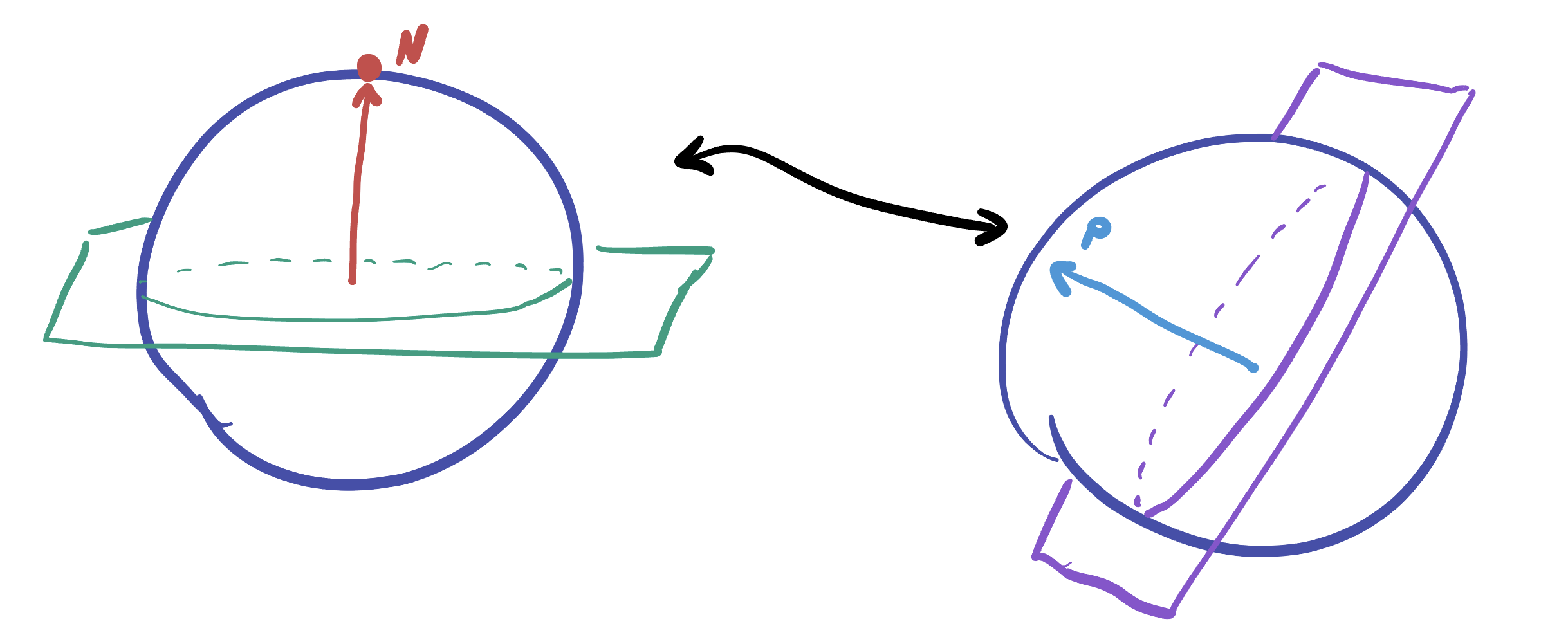
The equator is all the points which are orthogonal to the north pole \(N=(0,0,1)\)! Similarly, our great circle \(C\) is the intersection of \(\SS^2\) with some plane \(P\) - and this plane has a unit normal vector \(v\in\EE^3\), where we can describe \(C\) as the points of the sphere which are orthogonal to \(v\).
With this simple observation, we are already almost done! We know that we can find an isometry which takes \(N\) to \(v\) (Proposition 17.2), so call such an isometry \(\phi\). Because of how we constructed these isometries, we know \(\phi\) is an orthogonal transformation, and preserves angles. Thus, if \(p\) is any point of \(\SS^2\) orthogonal to \(C\), its sent to a point which is orthogonal to \(N\)! This means the circle \(C\) is sent to the equator, as required.
Now let \(R(x,y,z)=(x,y,-z)\) be the reflection in the equator that we used to prove it was a geodesic. From \(R\) and \(\phi\) we can build the isometry
\[\psi = \phi\circ R\circ \phi^{-1}\]
This takes \(C\) to the equator, reflects in the equator, and then returns the equator to \(C\). Thus any point on \(C\) is unchanged by \(\psi\), so \(C\) is a fixed curve by this isometry - its a geodesic!
The realization that great circles are geodesics has another nice corollary - it makes it easy for us to draw a line between any two points of the sphere! This was the content of Euclids’ axiom I, so we may say that this still holds on \(\SS^2\).
Remark 18.2. In modern mathematics, the ability to draw a geodesic between any two points of a space remains very important - spaces where you can do this are called geodesic metric spaces.
Proposition 18.1 Given any two points \(p\) and \(q\) of \(\SS^2\), its possible to draw a geodesic segment connecting them.
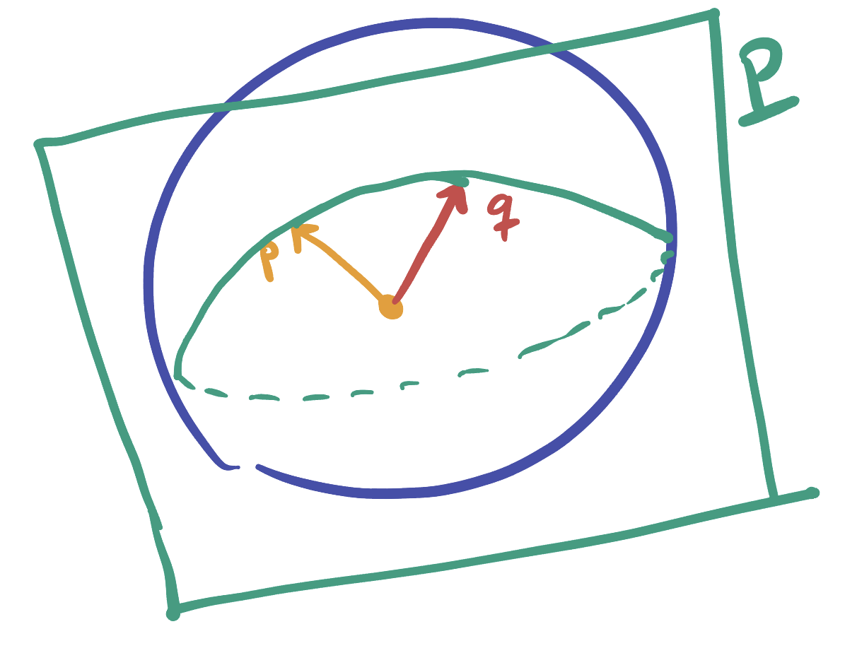
Proof. If \(p,q\) are two points of the sphere, form a plane \(P\) through the origin containing both \(p\) and \(q\). (When \(p\) is not exactly opposite \(q\) on \(\SS^2\) they are linearly independent, so this plane is just their span. If \(p=-q\) then you can take any plane you like containing the line of multiples of \(p\)). This plane intersects the sphere in a great circle containing both \(p\) and \(q\), so there is a geodesic of \(\SS^2\) that passes through \(p\) and \(q\).
Instead of describing geodesics as connecting two points, we can also describe geodesics in terms of their starting point and a starting direction. Like we did in Euclidean space, we can use Exercise 45 to see that given any point \(p\) and any unit tangent vector \(v\) on the sphere, there is a geodesic passing through \(p\) in direction \(v\) (use this exercise to translate the equator, which passes through \((1,0,0)\) with tangent \(\langle 0,1,0\rangle\) to \(p\) and \(v\) respectively).

18.1.2 Straightness on the Sphere
This section is suggested - but optional - reading, as we have already found all the geodesics above! But, while the definition of line of symmetry was the easiest to translate onto the sphere, its worth pausing a bit to talk about how we might define straightness here. In Euclidean space we said a curve was straight if its tangent vector did not change in time. But this definition will not do for \(\SS^2\)! Indeed, any curve whose tangent vectors do not change in time can be written as an affine equation, and none of these lie on the sphere!
What does “straight” mean on the sphere? It still means “does not turn”, but we must be careful since we are working with the sphere inside of \(\RR^3\), and all curves restricted to the sphere bend with the sphere itself.
Definition 18.3 (Spherical Acceleration) If \(\gamma\) is a curve on the sphere, its spherical acceleration at \(p\) is the projection of \(\gamma^{\prime\prime}\) onto the tangent space \(T_p\SS^2\).

This definition is precise, but not useful - we would like to have a formula which will let us compute the exact value of the spherical acceleration of any curve. And to get one - we need to do some Euclidean geometry! The key will be the ability to project a vector onto a plane.
Theorem 18.2 Let \(P\) be a plane in \(\EE^3\) with normal vector \(\vec{n}\). Then if \(v\in\EE^3\) is a vector (a point, thought of as a vector from the origin), the projection of \(v\) onto \(P\) is given by \[\mathrm{proj}(v)= v-\frac{v\cdot n}{n\cdot n}n\]
Proof. Let \(v\) be any vector, and \(P\) a plane with normal vector \(n\).

Our goal is to figure out how much of the vector \(v\) lies in the plane \(P\), and our approach will be kind of backwards. We will figure out how much of \(v\) is not in the plane, and the subtract this!
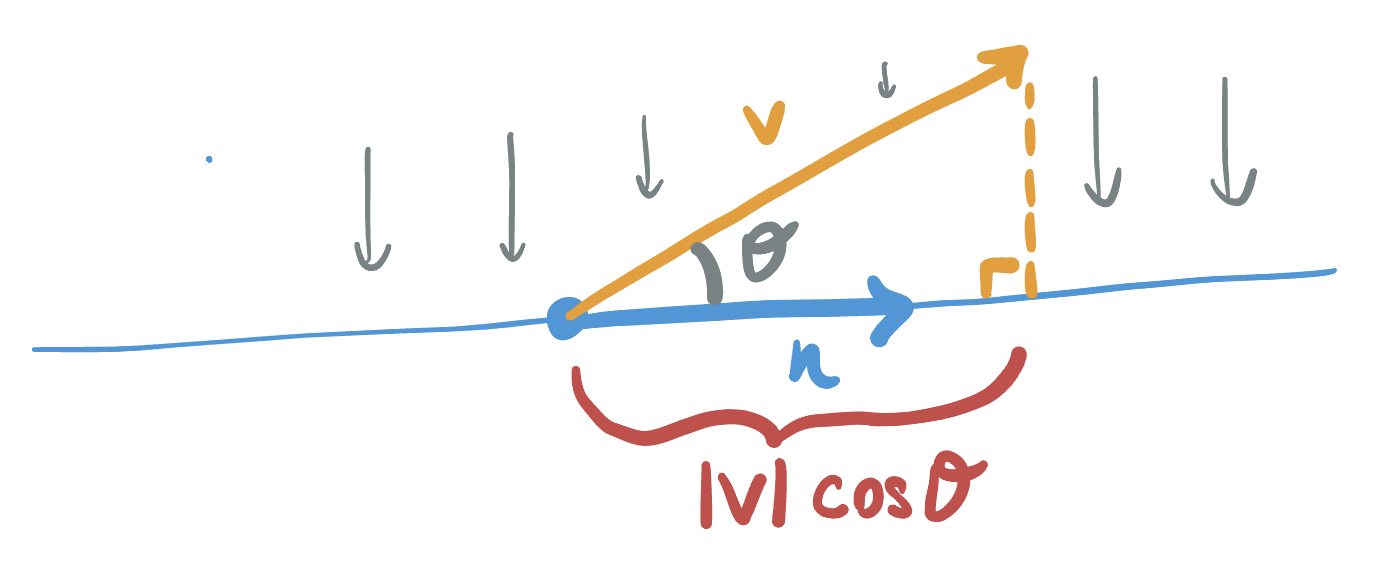
To figure out how much of \(v\) is not parallel to the plane \(P\), we need to figure out how much is in the direction of the normal vector \(n\). That is, we wish to compute the projection of \(v\) onto the line spanned by \(n\):

This is actually a problem of Euclidean plane geometry, which we can solve using angles and the dot product! Let’s look just in the Euclidean plane containing \(v\) and \(n\), where the projection of \(v\) onto \(n\) forms a right triangle with hypotenuse \(v\). From here, we can see the quantity we want is \(\|v\|\cos\theta\), where \(\theta\) is the angle between \(v\) and \(n\).
But, we also know that \(\cos\theta\) is defined in terms of the dot product!
\[\cos\theta = \frac{v\cdot n}{\|v\|\|n\|}\]
Thus, the projection onto \(n\) is
\[\|v\|\cos\theta = \|v\|\frac{v\cdot n}{\|v\|\|n\|}=\frac{v\cdot n}{\|n\|}\]
This is the length of the projection of \(v\) onto \(n\): what we need now is a vector in the direction of \(n\), which has this length. The solution? Just multiply by the unit vector in direction \(n\)!
\[\frac{v\cdot n}{\|n\|} \frac{n}{\|n\|}\]
This can be simplified algebraically, since we have two copies of \(\|n\|\) in the denominator now:
\[\frac{v\cdot n}{n\cdot n}n\]
Phew! But - this is the amount of the vector not in the plane. It’s exactly the part of \(v\) that we don’t care about! To get what we want, we need to subtract this from \(v\):
\[\proj = v-\frac{v\cdot n}{n\cdot n}n\]
It’ll be useful to note that this formula simplifies a bit if \(\|n\|=1\), to become just \[\mathrm{proj}(v)=v-\left(v\cdot n\right)n\]. This allows us to project onto any plane we wish in \(\EE^3\), so long as we know its normal vector. But our goal is to project onto the tangent plane to \(\SS^2\), so we can do even better, since we know exactly what the tangent spaces are. Indeed, if \(v\) is a vector in \(\EE^3\) based at a point \(p\) on the sphere, we can write down a projection map directly to the sphere:
Definition 18.4 (Projecting onto \(T_p\SS^2\).) If \(v\) is a vector in \(\EE^3\) based at \(p\), then its projection onto \(T_p\SS^2\) is \[\mathrm{proj}_{\SS^2}(v)=v-(v\cdot p)p\]
Indeed, at the point \(p\in\SS^2\), the tangent space is the set of all vectors orthogonal to \(p\) - so the normal vector to \(T_p\SS^2\) is just \(p\) itself! This
Corollary 18.2 (Spherical Acceleration) Given a curve \(\gamma(t)\) on \(\SS^2\), its spherical acceleration is \[\begin{align*} \mathrm{acc}_\gamma(t)&=\mathrm{proj}_{\SS^2}(\gamma^{\prime\prime}(t))\\&=\gamma^{\prime\prime}(t)-\left(\gamma^{\prime\prime}(t)\cdot\gamma(t)\right)\gamma(t) \end{align*}\]
Now we can formally define what it means for a curve on the sphere to be straight. Because this process produces an equation that \(\gamma\) has to satisfy to be a geodesic, it is called the geodesic equation and versions of it are fundamental to modern geometry - from the sphere to hyperbolic space to black holes and beyond.
Definition 18.5 (The Geodesic Equation for \(\SS^2\)) A curve on the sphere is a geodesic if its spherical acceleration is zero. That is, \(\gamma\) is a geodesic if \(\mathrm{acc}_\gamma(t)=0\), or
\[\gamma^{\prime\prime}(t)-\left(\gamma^{\prime\prime}(t)\cdot\gamma(t)\right)\gamma(t)=0\]
Remark 18.3. This looks pretty daunting - at least in comparison to what we had to do in Euclidean space! There, our equation for straightness was just \(\gamma^{\prime\prime}=0\), which we could solve by hand using Calculus I. This equation howver is much more complicated! If we write out \(\gamma\) in terms of components \(\gamma(t)=(x(t),y(t),z(t))\) we can expand this equation all the way out into a system of three equations, for \(x,y,z\): \[\gamma^{\prime\prime}=(\gamma^{\prime\prime}\cdot\gamma)\gamma\] Writing \(\gamma(t)=(x(t),y(t),z(t))\) we can fully write this out as a vector equation \[\pmat{x^{\prime\prime}\\ y^{\prime\prime}\\z^{\prime\prime}}=\left(\pmat{x^{\prime\prime}\\ y^{\prime\prime}\\z^{\prime\prime}}\cdot \pmat{x\\ y\\ z}\right)\pmat{x\\ y\\ z}\] And, this vector equation is really just a system of three equations, which I’ll write out below (expanding the dot product, which is the common factor multiplied to all of them): \[\left\{\begin{matrix} x^{\prime\prime}=\left(x^{\prime\prime}x+y^{\prime\prime}y+z^{\prime\prime}z\right)x\\ y^{\prime\prime}=\left(x^{\prime\prime}x+y^{\prime\prime}y+z^{\prime\prime}z\right)y\\ z^{\prime\prime}=\left(x^{\prime\prime}x+y^{\prime\prime}y+z^{\prime\prime}z\right)z \end{matrix}\right\}\] In less symmetrical geometries, the only way forward from here is to actually solve this system of coupled differential equations! However, luckily for the sphere there’s plenty of symmetry, and we can avoid this mess.
Now its our goal to show that the collection of curves which are straight on the sphere is the same as the collection which are fixed by some symmetry: that just like in Euclidean space, these two notions of geodesic coincide!
Theorem 18.3 (Straight Curves on the Sphere) All great circles are straight - they have zero spherical acceleration.
Proof. First, we start with the equator \(e(t)=(\cos t,\sin t,0)\). We need to show that \(\mathrm{acc}_e(t)=0\), by computing
\[\acc_e = e\pp - (e\pp \cdot e)e\]
Computing we see \(e\pp = -e\) since its components are sinusoids, and so \(e\pp\cdot e =(-e)\cdot e =-(e\cdot e)=-1\) because \(e\) lies on the unit sphere. Plugging this in, we see that \(\acc_e = e\pp - (-1)e = e\pp +e\) But now we can use once more that \(e\pp = -e\)! Thus \[\acc_e = e\pp +e = -e+e=0\] So, the equator experiences no spherical acceleration, and thus is straight as claimed.
Next, we need to show this for an arbitrary great circle \(c(t)\). Let \(P\) be the plane containing this great circle, and \(p\) be its normal vector. Then since we know there is an isometry of \(\SS^2\) taking \(N\) to \(p\), we have an isometry taking \(c(t)\) to the equator \(e(t)\), and thus its inverse is an isometry taking \(e(t)\) to \(c(t)\): because this isometry is an orthgonal transformation I will represent it by its matrix \(A\), so we can write
\[c(t)=Ae(t)\]
Where the juxtaposition \(Ae\) is matrix multiplication. Now we wish to use the fact that we know \(e\) is straight, to show that \(c\) is too. Our overall goal is to compute \(\acc_c(t)\), so let’s write this out:
\[\begin{align*} \acc_c &= c\pp - (c\pp \cdot c )c\\ &=(Ae)\pp - ((Ae)\pp\cdot (Ae))(Ae) \end{align*}\]
To simplify, we need to compute the second derivative of the composition \(Ae(t)\). Let’s just take one derivative at a time: by the chain rule
\[(Ae(t))^\prime = DA_{e(t)}e^\prime(t)\]
and, since \(A\) is a linear map it is its own derivative: \(DA_{e(t)}=A\)! Thus this simplifies to the statement “you can pull \(A\) out of the derivative”, and similarly upon differentiating once more:
\[(Ae(t))^\prime = Ae^\prime(t)\,\,\implies\,\,(Ae(t))\pp = Ae\pp(t)\]
Plugging this into our spherical acceleration formula, we find
\[\acc_c = Ae\pp - ((Ae)\pp\cdot (Ae))Ae\]
There’s still plenty of simplification to be done! The first order of business is to deal with the dot product here. Since \(A\) is an isometry it preserves the dot product by definition:\((Av)\cdot (Aw)=v\cdot w\). Applying this in our case we can remove the \(A\)s above, resulting in
\[Ae\pp - (e\pp \cdot e)Ae\]
Now, whatever \(e\pp\cdot e\) is, its just a number for each value of \(t\). Sine \(A\) is a linear map, we can pull it inside the map, and then use linearity to combine everything together:
\[\begin{align*} Ae\pp - (e\pp \cdot e)Ae&= Ae\pp -A((e\pp\cdot e)e)\\ &= A(e\pp-(e\pp\cdot e)e) \end{align*}\]
But now we are done! Look at what we are applying the linear map \(A\) to here: its nothing other than the spherical acceleration of the equator \(e\)! And we already know that \(e\) is straight, so this is zero. Finally, since \(A\) is a linear map it sends zero to zero, and so
\[\acc_c = A(\acc_e)=A(0)=0\]
Thus \(c\) is also straight!
This argument was pretty long and algebraic, more so than many of the more geometric arguments we’ve given throughout the course. I wanted to present it this way to show the power of all the tools we built: we managed to prove something about the curve \(c\) using nothing but properties of isometries and calculus: this is how many arguments in modern geometry proceed.
18.1.3 Distance on the Sphere
Now that we know the geodesics of the sphere, we can really get geometry moving by deriving the distance function.
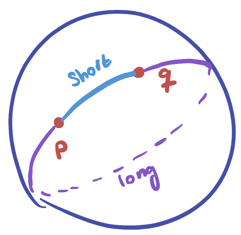
But there is one subtlety we have to confront first. In Euclidean space, we proved that given any two points there was a unique line segment connecting them. And then we took the length of this line segment as the distance between them. But this seemingly simple fact is false on the sphere! Here geodesics are circles, and given two generic points there are actually two ways to connect them with segments of a great circle - going around the circle one way, or the other!
Exercise 18.1 True or false, between any two points on the sphere there are exactly two geodesic segments connecting them. (Can there ever be more? If so, when and how many?)
Of course, in general one of these is shorter than the other, and this does not pose any big theoretical problem. We just have to amend our terminology a bit, as in the plane we found the distance between two points was the length of the line segment connecting them.
Definition 18.6 The distance between two points \(p\),\(q\) on the sphere is the length of the shortest curve connecting them. This is the length of the shorter of the geodesic segments defined by the great circle passing through \(p\) and \(q\).
Believe it or not, we’ve already done all the rest of the hard work, and the distance formula is sitting here waiting for us to realize it! First, let’s consider two points on the equator. Since the equator is just the unit circle in the Euclidean plane \((x,y,0)\), these two points determine two vectors on the unit circle, and what we want to know is the length of arc between them.
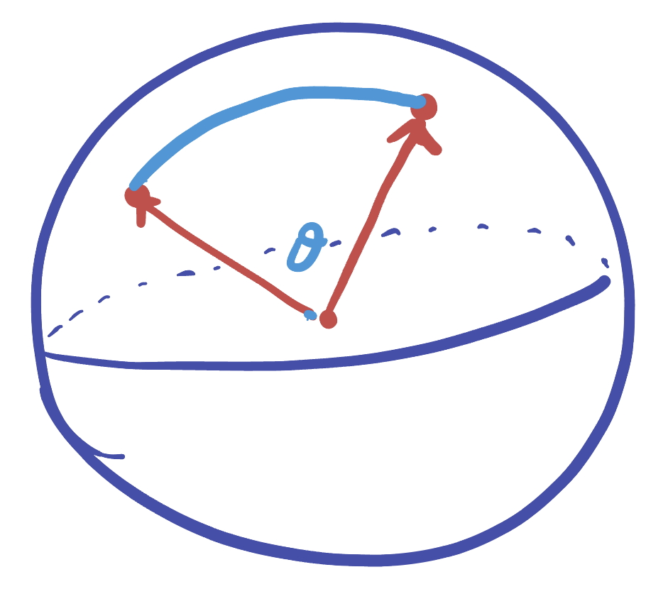
But this is the definition of angle! So, in spherical geometry, we have an beautiful relationship between distance and angle:
The distance between \(p\) and \(q\) on \(\SS^2\) is the same as the angle between them as vectors in \(\EE^3\).
Even better, we spent plenty of time working out exactly how to measure angles quantitatively, in the end discovering a nice relationship between the angle \(\theta\) and the dot product. Furthermore, while we developed all of this material just in the plane, isometries do not change lengths (and thus do not change angles), so we can take this result from the Equator and apply it to any great circle on \(\SS^2\) via an isometry:
Theorem 18.4 let \(p,q\) be two points on \(\SS^2\). Then the distance between them is equal to \[\dist(p,q)=\arccos(p\cdot q)\]
Just like the distance formula in \(\EE^2\) was the key to unlocking the rest of geometry (circles, trigonometry, and \(\pi\)), so is this distance formula, to unlocking the rest of the geometry of the sphere.
18.2 Circles
A circle is defined to be the set of points which are the same distance (the radius) from a fixed point (the center). We wish to study these curves in spherical geometry, now that we have the distance function available to us.
Like many things, its easiest to start working about a familiar point (the origin in \(\EE^2\), the north pole in \(\SS^2\)) and generalize beyond that using isometries.
Proposition 18.2 (Circles about the North Pole) The circle of radius \(r\) about \(N=(0,0,1)\) in \(\SS^2\) is given by the points \[C_{N,r}=\{(x,y,\cos(r))\in\SS^2 \}\]
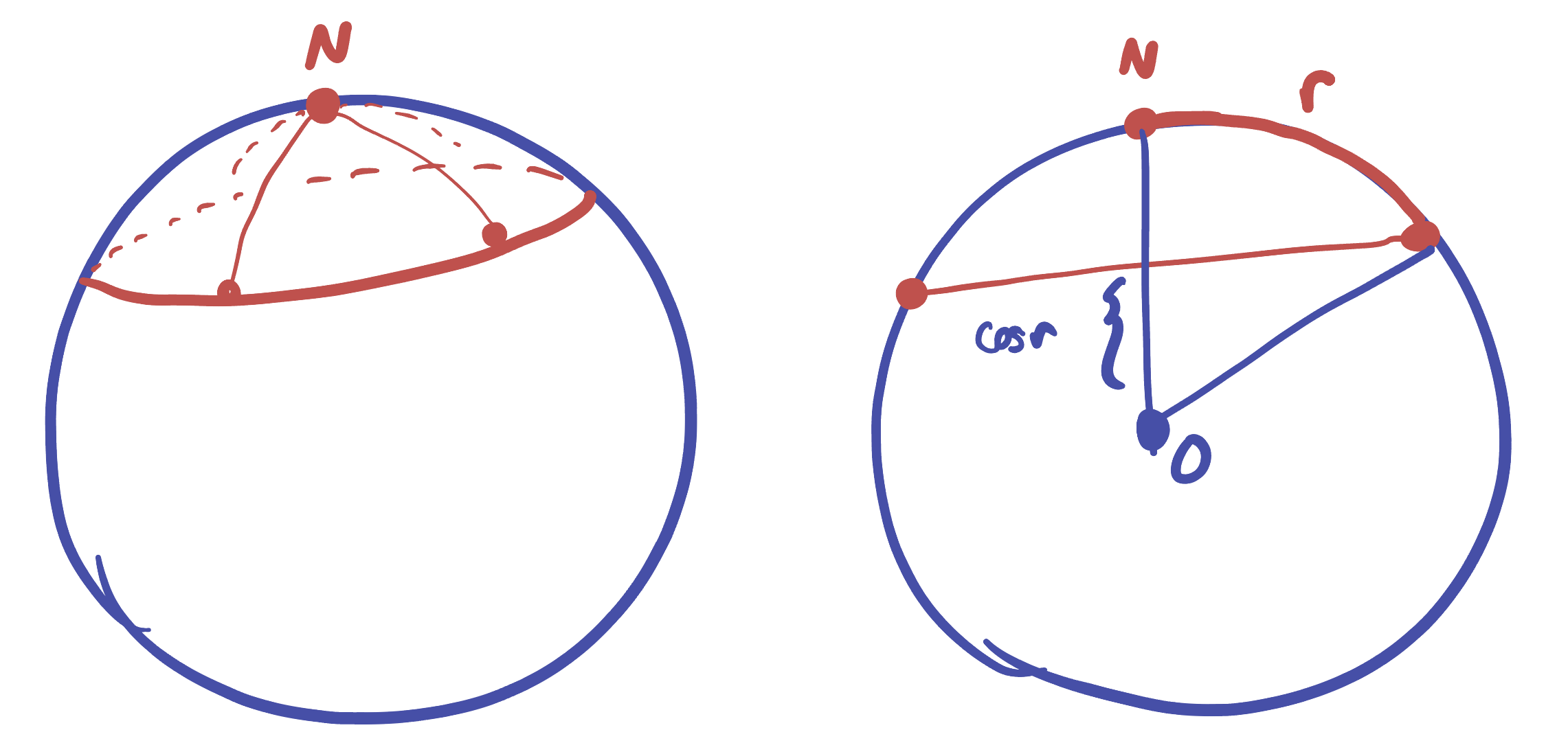
Proof. We just need to see these are the points which lie at distance \(r\) from \(N\) along \(\SS^2\). The crucial point is that we are measuring distances along the sphere, not in \(\EE^3\), so \[\begin{align*}d((x,y,z),N)&=\arccos((x,y,z)\cdot N)\\ &=\arccos((x,y,z)\cdot (0,0,1))\\ &=\arccos(z) \end{align*}\] Thus, for \((x,y,z)\) to lie on the circle it must (1) be a point on the sphere and (2) have \(\arccos(z)\) equal to the radius - equivalently \(z=\cos(r)\).
Corollary 18.3 (Circles on the Sphere) Circes are intersections of planes which do not pass through the origin with the sphere.
We see this is true in the case centered on \(N\), as the circle consists of all points with a fixed constant \(z\) coordinate: this is just a horizontal plane intersecting the sphere! To argue the general case, we use isometries: we know that any great circle can be taken to any other by an orthogonal transformation of \(\EE^3\) - and these are linear maps so they take planes to planes.
Thus, starting from a circle around the north pole cut out by a horizontal plane, moving this plane by an orthogonal transformation takes this plane to another plane, and its intersection to another circle!

We have come across two distinct curves on the sphere which can be described as the intersections of the sphere with planes. First, we had the great circles, corresponding to planes through the origin, which are the spherical analog of straight lines. These second ones are planes not through the origin, which correspond to geometric circles. What is going on here - how can these two different classes of curves seem so similar? After all, just shifting a plane slightly downwards can turn it from something curved (a circle) to something straight (a geodesic).

In fact, this is not as strange as it seems at first, and there’s a sort of analog happening already in the Euclidean plane. Here, as a circle’s radius grows larger and larger, the circle itself appears ‘straighter’ nearby. The difference is that this only becomes exact in the limit where the circle’s radius goes to infinity, whereas on the sphere, this straightening of circles happens at a finite radius: \(r=\tau/4\).
18.2.1 Area and Circumference
Now that we know what the circles on \(\SS^2\) are, its time to get quantitative and study their radii and circumference. In Euclidean space, we used isometries to show that any two circles of the same radius could be brought to one another. This same argument goes through without change on the sphere:
Exercise 18.2 There is an isomery taking any circle of radius \(r\) to any other.
This was our first step to understanding the length constant \(\tau\): because isometries do not change lengths, this told us that every circle of radius \(r\) has the same circumference. And now, we know the same thing for the sphere! But the key step to understanding \(\pi\) and \(\tau\) was figuring out how circles of different radii were related.
Theorem 18.5 The only similarities of the sphere are isometries: there are no maps which non-trivially uniformly stretch infinitesimal distances.
Proof. Let \(\sigma\) be such a similarity, which scales all infinitesimal lengths by \(k\). Then \(\sigma\) preserves the dot product, and sends infinitesimal squares to other squares, expanding their area by \(k^2\). This doesn’t sound like a problem, until you remember that the entire spherical universe has a finite area!
The area of the unit sphere \(\SS^2\) is \(4\pi\), and if \(\sigma\colon\SS^2\to\SS^2\) is the supposed similarity above, it would take this area to an area \(4\pi k^2\). But - this map is supposed to take the sphere to the sphere (it can’t take it to a larger sphere in \(\EE^3\): that’s a different space)!
Thus, since the image is the same sphere we know that its area is still \(4\pi\), so \(4\pi k^2=4\pi\), or \(k^2=1\). Thus, the only possibility is \(k=1\) (as \(k\) is the scaling factor, a positive number), which corresponds to isometries.
This simple fact - that \(\SS^2\) does not have any similarities - has profound consequences for its geometry. First off, it assures there’s no hope of generalizing our proof that circumference/radius is a constant. Of course, this does not guarantee that its not a constant (perhaps we just need a different style of argument). To see what’s really going on, we need to do some computations!
Before diving into the general case, its helpful to look at a couple of special cases: we will consider circles of very small radius, great circles, and circles of very large radius.


If the radius \(r\) is very small, then the circle itself fits within a very small region of \(\SS^2\), and small regions of space are well-approximated by their tangent plane. Thus, we expect that small circles are very close to being Euclidean circles (think about drawing a circle on the sidewalk, which is a small portion of the spherical earth). Being nearly Euclidean, we expect their ratios of circumference to diameter to be very close to the Euclidean value of \(\tau\), or \(2\pi\approx 6.28\).
Now, what about a great circle? For specificity, let’s consider the equator as a circle about the north pole. The radius is a quarter of a way around the sphere (half way would be from the north pole to the south pole, and the north pole to the equator is half of that). But the circumference is one full revolution around the sphere: so this means that circumference over radius is \(\frac{\tau}{\tau/4}=4\)! This shows us a very important fact - the sphere’s analog of \(\tau\) (the ratio of circumference to radius) cannot be a constant! It takes on values slightly larger than \(6\) for small circles, but takes on the exact value of \(4\) for a great circle.
How small can this ratio get? Consider a circle of a very large radius: close to \(\pi\) - so the radius runs from the north pole all the way down to something close to the south pole. The set of all points which lie at this distance from \(N\) is short curve near the south pole. So here the ratio of circumference to radius is a small circumference to a big radius - its a very small number!
These qualitative considerations not only show us that the spherical analog of \(\tau\) is not a constant, but also that we expect it to be able to take on any values between 0 and 6.28. But to get more precise than this we actually need to sit down and do some calculations…
Proposition 18.3 Show the circumference of the circle of radius \(r\) is \[2\pi\sin(r)\]
Proof. We know already that the circle of radius \(r\) about the north pole \(N\) is contained in the plane \(z=\cos(r)\). But this is a Euclidean plane! So, we can measure this circles circumference using Euclidean geometry.

Say its radius in the plane is \(d\) (note its radius on \(\SS^2\) is \(r\), but this lies on the sphere, not on the plane). Then we can use our understanding of Euclidean circles to see \(C=2\pi d\). But what is \(d\)? Looking at a side view of our configuration, \(d\) is the opposite side of a right triangle with angle \(r\) inside a unit circle:
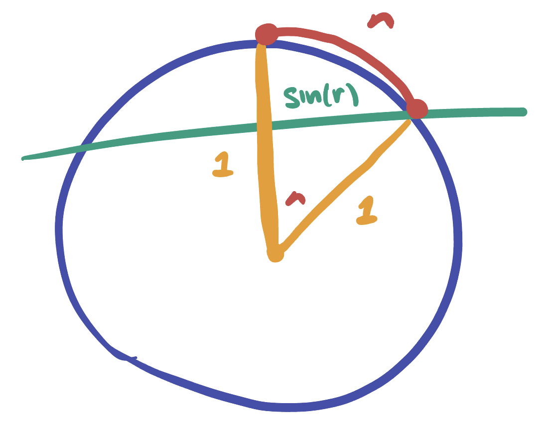
Thus, \(d=\sin(r)\) and so \(C=2\pi \sin(r)\) as claimed.
Corollary 18.4 (There is no length constant.) There is no single number like \(\tau\) which is a universal constant for all circles on the sphere, like there was for circles on the plane.
Proof. Recall we defined the function \(\tau(r)\) to be the circumference of a circle of radius \(r\), divided by its radius. In Euclidean space we found this was a constant, independent of circle. But on the sphere, we see
\[\tau(r)=\frac{2\pi\sin(r)}{r}\] which is not constant!
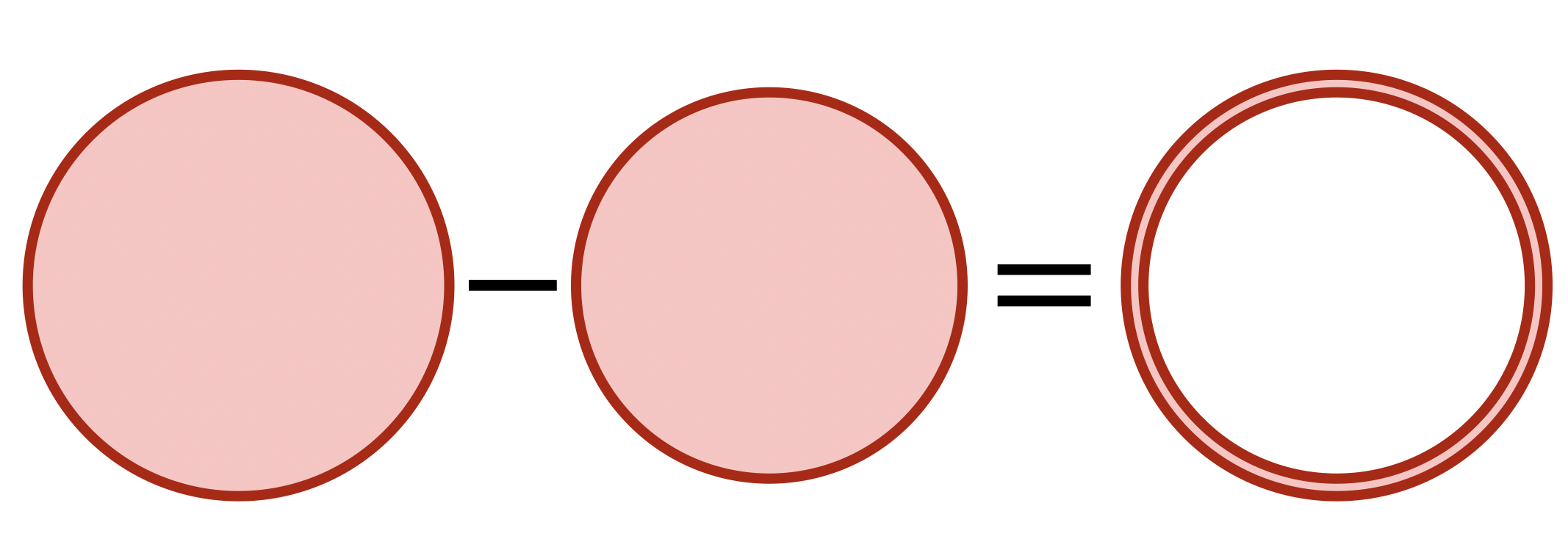
This pattern continues for area, where we show there is also no analog of \(\pi\) by seeing that areas of circles do not grow quadratically with radius. But first - how do we find the area of a circle on the sphere? We need to to use integration, to add up all the small infinitesimal area elements! Here the easiest way to do this is to invert our relationship between area and circumference discovered in Theorem 16.4. This same logic applies on the sphere, showing circumference to be the derivative of area.
\[\frac{d}{dr}\mathrm{area}(r)=\lim_{h\to 0^+}\frac{\mathrm{area}(r+h)-\mathrm{area}(r)}{h}\approx\frac{\mathrm{circ}(r)\cdot h}{h}=\mathrm{circ}(r)\]
Thus, if \(A^\prime(r)=C(r)\), we can recover the formula for area via integration:
\[A(r)=\int_0^r C(r)dr\]
Proposition 18.4 (Area of a Circle) The area of a circle of radius \(r\) on \(\SS^2\) is
\[A(r)=4\pi \sin^2(r/2)\]
Proof. This is just an explicit computation, using the result of ?exr-sphere-circle-circumference.
\[A(r)=\int_0^r 2\pi\sin(r)dr\] \[=-2\pi\cos(r)\Bigg|_0^r=2\pi(1-\cos(r))\] \[=4\pi \frac{1-\cos r}{2}=4\pi\left(\sqrt{\frac{1-\cos r}{2}}\right)^2\] \[=4\pi \sin^2\left(\frac{r}{2}\right)\] Where, in the last two lines, we have used the half-angle formula to simplify our original answer, into a form that looks more similar to what we are used to in the Euclidean case.
Exercise 18.3 Use the series expansion of \(\sin x\) to give the first few terms of a series expansion of \(A(r)\). Show that the first nonzero term is \(\pi r^2\): this means when \(r\) is small, \(A(r)\) is approximately \(\pi r^2\). What does this mean geometrically?
18.3 Three Dimensions
The three dimensional version of spherical geometry is given by the surface of the four dimensional ball, just as the two dimensional sphere is the surface of the ball in three dimensions.
While it is hard to directly picture this space in four dimensions, its possible to compute things directly analgously to what we did above.
Definition 18.7 (Points and Tangent Spaces) The points of \(\SS^3\) are the four tuples of length \(1\) in \(\EE^4\): \[\SS^3=\{(x,y,z,w)\mid x^2+y^2+z^2+w^2=1\}\] A vector \(v=\langle v_1,v_2,v_3,v_4\rangle\) is tangent to \(\SS^3\) at \(p=(x,y,z,w)\) if it is orthogonal to \(p\): \[T_p\SS^3=\{v\mid v\cdot p = 0\}\]
Much of the mathematics of \(\SS^2\) carries over to \(\SS^3\) with little change. In particular - we can find the geodesics by finding the straight curves, and see that they are again just great circles.
Theorem 18.6 (Geodesics) Geodesics on \(\SS^3\) are great circles: they are intersections of 3-dimensional hyperplanes in \(\RR^4\) with the unit sphere. For example \(e(t)=(\cos t,\sin t, 0,0)\) is a geodesic.
Exercise 18.4 Prove this: write out what it means to have zero tangential acceleration, and prove that \(e(t)=(\cos t,\sin t, 0,0)\) is such a curve.
Because the geodesics are the same class of curves, we can measure distance in the same way - its an arc length of a circle, so distance equals angle!
Theorem 18.7 If \(p,q\in\SS^3\) then the distance between \(p\) and \(q\) is given by
\[\dist(p,q)=\arccos(p\cdot q)\]
Exercise 18.5 Let \(N=(0,0,0,1)\) be the north pole of \(\SS^3\). What are teh points of the sphere of radius \(r\) about \(N\)?
Exercise 18.6 What is the surface area of a sphere of radius \(r\)? What is its volume?