27 Geometry
Now that we have a concrete model of hyperbolic space (actually, many of them), its time to put them to work, and prove some things about hyperbolic space. Of course we already know a lot - we followed many geometric formulas directly through the limiting procedure! But these formulas speak of geodesics and circles, and we don’t know what these things look like in our models, so it’s hard to begin using these facts to do anything! We will remedy that gap in this chapter, and in the end, prove that hyperbolic space satisfies Euclid’s postulates 1-4 while failing the fifth.
27.1 Homogenity & Isotropy
As we have for both the plane and the sphere, we begin our journey by investigating the symmetries of hyperbolic space. This will be our first foray into using the two models to inform one another, and switching back and forth whenever is convenient, whether than being tied down to a single way of calculating.
As we saw in defining the disk model, its easy to see that rotations about its center are isometries (though its hard to see that there are any other symmetries at all, at first!)
Proposition 27.1 (Rotations of Disk are Isometries) Euclidean rotations of the plane about the origin restrict to isometries of the Disk Model of \(\HH^2\).
Proof. Rotation isometries of the plane do not change the distance of a point from the origin, and they do not affect the Euclidean dot product of two tangent vectors. Because the hyperbolic disk dot product is just the Euclidean one rescaled by a function of distance from the origin, it is also unchanged by a rotation, so these rotations are hyperbolic isometries!
To find more isometries, we can switch our viewpoint and take a look in the Half Plane model. Since isometries are maps which preserve the infinitesimal dot product, we can use the fact that the scaling factor here only depends on \(y\) to find some new isometries of hyperbolic space.
Proposition 27.2 (Horizontal Translation is an Isometry) Any euclidean horizontal translation \((x,y)\mapsto (x+a,y)\) is an isometry of the upper half plane model.
Proof. Translations are Euclidean isometries, so they preserve the Euclidean dot product. But horizontal translations also preserve the \(y\) coordinate, and hence the scaling factor. Thus, they preserve the hyperbolic dot product as well.
These isometries are different than those that we discovered before, as they move the point \((0,1)\) (which is where the origin of the disk was sent), whereas our earlier-discovered isometries fixed the origin (and hence would would fix \((0,1)\) here).
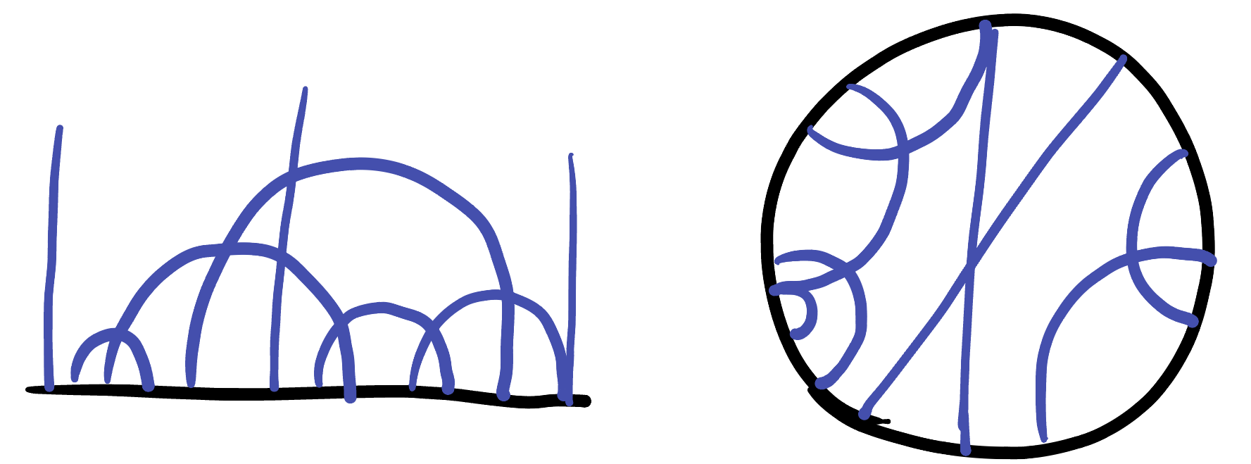
We can see what these look like in both models, using the pictures we developed above. Vertical lines in the Half Plane correspond to circles through \((0,1)\) on the boundary in the Disk Model, and our new isometries move these curves to one another.
Other translations of the Half Plane are not isometries, as any map that changes the \(y\) coordinate is going to change the scaling factor applied by the dot product:
Example 27.1 The map \(\tau(x,y)=(x,y+1)\) is not an isometry of the Half Plane model.
Let \(v,w\) be two vectors based at \((x,y)\) in the upper half plane: then their hyperbolic dot product is
\[(v\cdot w)_{\HH^2} = \frac{v_1w_1+v_2w_2}{y^2}\]
The derivative \(D\tau\) of any translation is the identity, so \(D\tau v= v\) and \(D\tau w = w\), but now based at \((x,y+1)\) which means their new dot product is
\[((D\tau v)\cdot (D\tau w))_{\HH^2}=\frac{v_1w_1+v_2w_2}{(y+1)^2}\]
This is a different number so the dot product was not preserved, and the map was not an isometry.
We can see in this example what went wrong however: we moved vertically (increasing the denominator) without changing the vectors (leaving the numerator the same). Instead, when we
Proposition 27.3 (Homothety is an Isometry) Let \(\lambda>0\). Then the Euclidean similarity \(s(x,y)=(\lambda x, \lambda y)\) is an isometry of the Half Plane model of hyperbolic space.
Proof. Like the example, we just compute: here the derivative \(Ds\) is just scaling by \(\lambda\), so our vectors \(v\) and \(w\) at \((x,y)\) go to the vectors \(\lambda v\) and \(\lambda w\) at \((\lambda x,\lambda y)\). In the new dot product, the numerator is multiplied by \(\lambda^2\) (one \(\lambda\) from each vector), and the denominator is multiplied by \(\lambda^2\), so they cancel out:
\[\begin{align*}((Ds v)\cdot (Ds w))_{\HH^2}&=\frac{\lambda v_1\lambda w_1+\lambda v_2\lambda w_2}{(\lambda y)^2}\\ &=\frac{\lambda^2(v_1w_1+v_2w_2)}{\lambda^2y^2}\\ &=(v\cdot w)_{\HH^2} \end{align*}\]
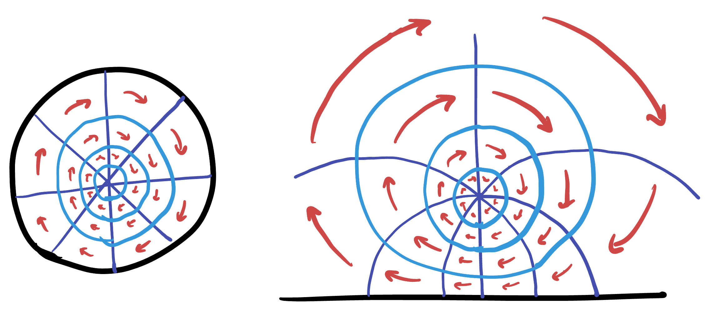
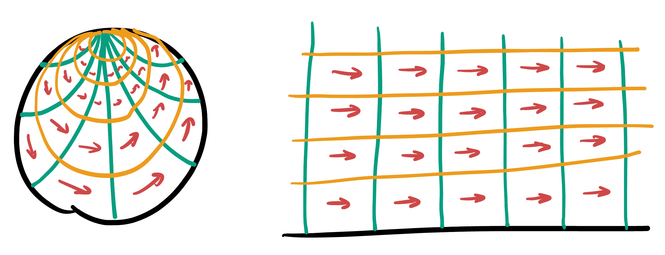
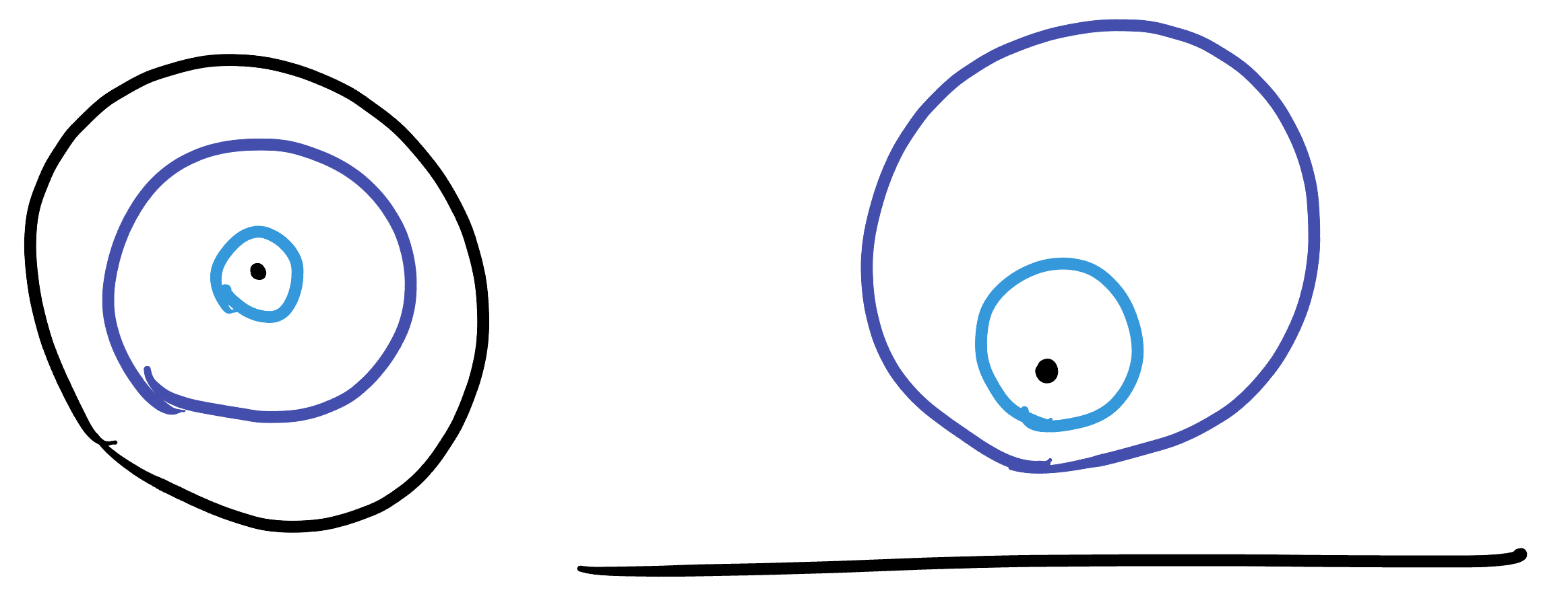
What does this kind of isometry look like in our two models? We understand well what it looks like through our euclidean eyes in the Half Plane: its just a similarity of the plane! But while it looks like points are getting farther apart here, they’re not. This is an isometry after all, so it preserves hyperbolic distances! The fact that it looks to be expanding is just a consequence of the fact that distances are artificially short-looking near the bottom, and artificially long towards the top. But what about in the disk model?
![]()
We’ve now discovered enough isometries to prove rigorously that hyperbolic geometry is both homogeneous and isotropic:
Exercise 27.1 (\(\HH^2\) is Homogeneous) There is an isometry taking any point of hyperbolic space to any other.
Next, we want to use this to see that space is isotropic: that about any point, there is a rotation by any amount. Here we may wish to switch over to the Disk Model, brining with us the fact that we just proved space is isotropic (even though we haven’t bothered to write down what those isometries look like in the disk). We know we can rotate by any angle we like about \(O\), and now we also know that its possible to move \(O\) to any arbitrary point \(p\). So, what do we do? We translate \(p\) to \(O\) do any rotation we like, and then translate back of course! Conjugation saves the day.
Corollary 27.1 (\(\HH^2\) is Isotropic)
This is enough to see that Euclid’s Postulate 4 is true for hyperbolic space: remember that Euclid’s phrasing all right angles are equal was the original way of saying homogeneous and isotropic.
27.2 Geodesics
We’ve been able to track down a couple curves in the various models that certainly must be geodesics - reasoning from watching what happens to great circles on the sphere under our transition. But we are still lacking in two things: (1) a rigorous proof, done in hyperbolic geometry itself, that these are in fact distance minimizing and more importantly (2) a classification of what all the geodesics are. We remedy this below, with computations that should feel very analogous to both the Euclidean and spherical cases.
Proposition 27.4 (Vertical Lines are Geodesics) In the Half Plane model, the vertical curve \(\gamma(t)=(0,t)\) is minimizing between any two points.
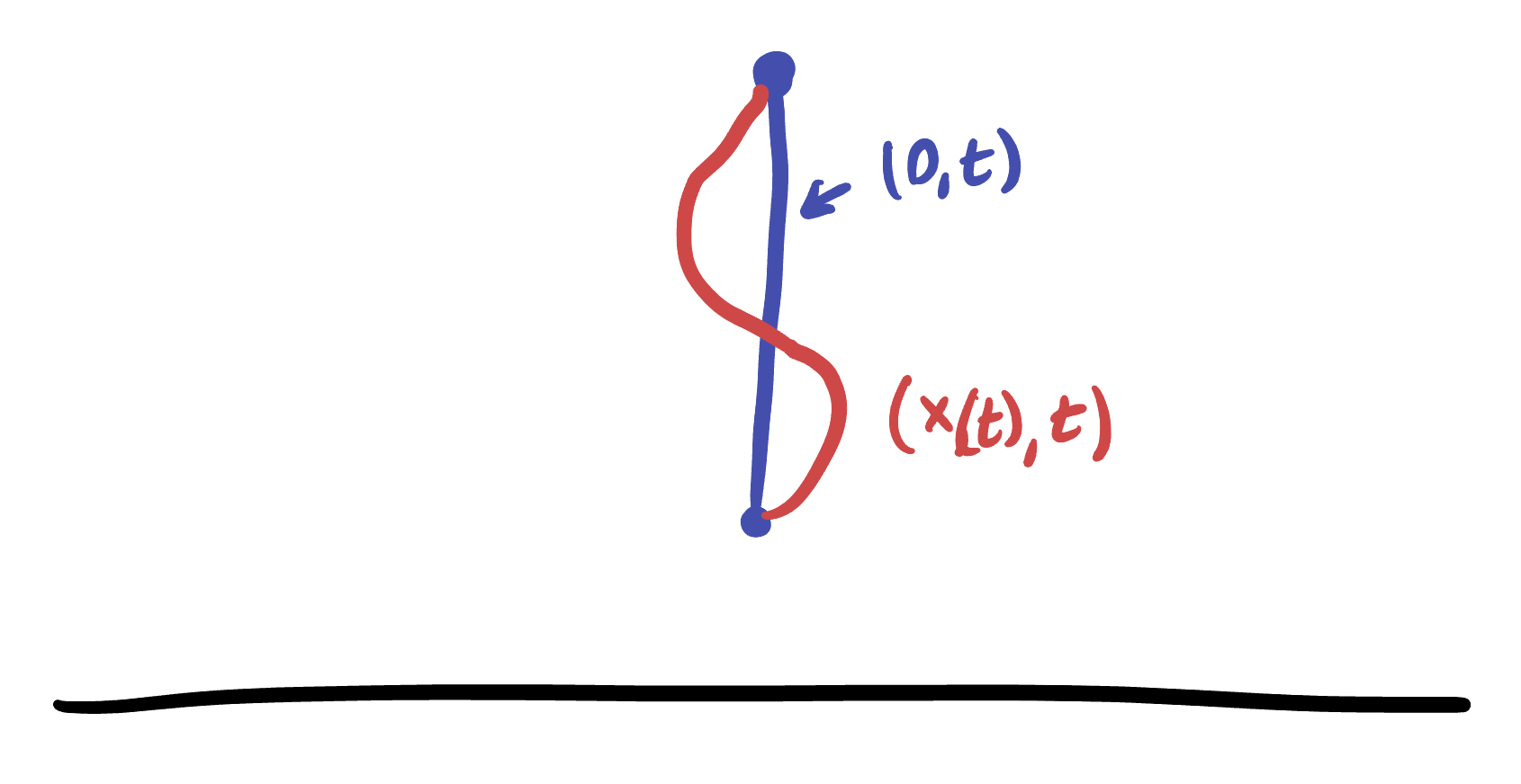
Proof. Consider the endpoints \((0,a)\) and \((0,b)\), and let \(\alpha(t)=(x(t),t)\) be any other curve between these for \(t\in[a,b]\). Then \(\alpha^\prime = \langle x^\prime, 1\rangle\) based at \((x,t)\) so its infinitesimal length is
\[\|\alpha^\prime\|=\frac{\sqrt{(x^\prime)^2+1}}{t}\]
We can do our usual trick, and notice that whatever \(x^\prime\) is, we know its square is positive, so we certainly have
\[\|\alpha^\prime\|\leq \frac{1}{t}\]
But this is exactly the infinitesimal lenght of \(\gamma\), since \(\gamma^\prime=\langle 0,1\rangle\). Thus we can integrate this inequality to find \[\|\gamma^\prime\|\leq\|\alpha^\prime\|\,\,\implies\,\,\int_a^b \|\gamma^\prime\|dt\leq \int_a^b\|\alpha^\prime\|dt\] \[\implies \len(\gamma)\leq\len(\alpha)\]
Given that these curves are distance minimizers, we can directly find the distance function between vertically separated points:
Corollary 27.2 (Vertical Distance Formula) The distance between \((0,a)\) and \((0,b)\) is \(\log(b/a)\).
Proof. This is just an integral of the infinitesimal length of \(\gamma(t)=(0,t)\) from \(t=a\) to \(t=b\):
\[\mathrm{length}(\gamma)=\int_a^b \frac{1}{t}dt=\log(t)\Big|_a^b=\log(b)-\log(a)=\log\left(\frac{b}{a}\right)\]
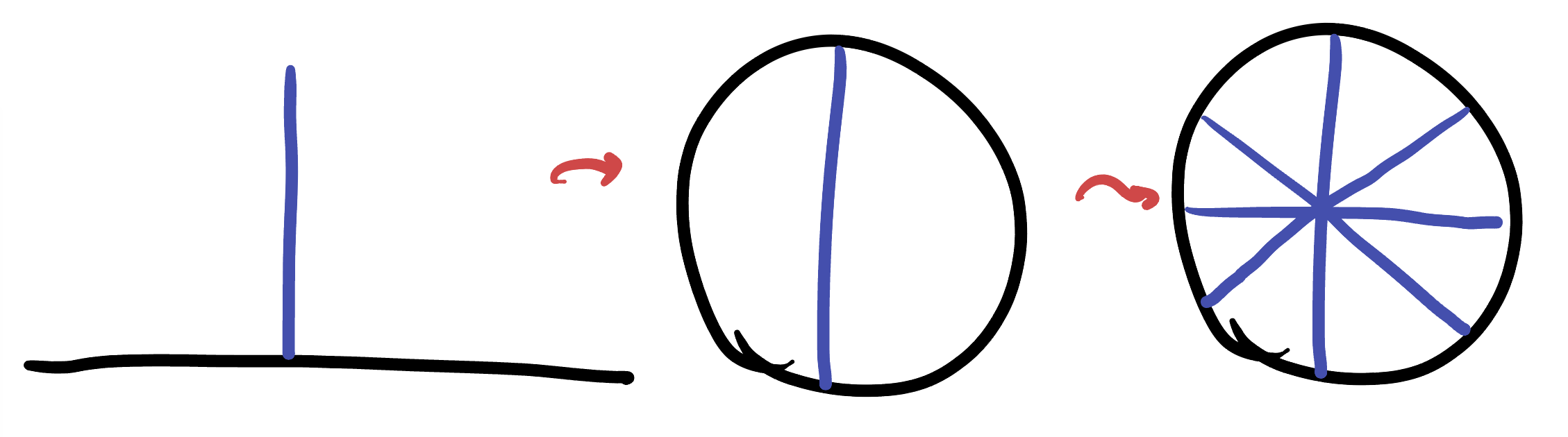
This tells us that all vertical lines are geodesics in the half plane model. And we can transfer this information over to the Disk Model to learn about some of the geodesics there. The vertical line through \((0,1)\) goes to a diameter of the unit disk as we can see by direct computation, plugging in \((0,t)\). Then, since we know the unit disk as rotations as isometries, we can see that all diameters of the disk are geodesics.
Next, we can transfer this information back to the Half Plane. Consider just a horizontal diameter of the disk. After transferring back, we know this must go to a generalized circle through \((0,1)\), and that it must intersect the vertical line at a right angle. This doesn’t leave us many options: in fact, it uniquely specifies it! It must be the top half of the unit circle.
So, this half circle is a geodesic. But as soon as we know that, we can use the fact that horizontal translations and similarities of the plane are isometries to get that all half circles orthogonal to the real line are geodesics, and all vertical lines as well.

Theorem 27.1 (Geodesics in the Half Plane Model) The geodesics in the disk model are arcs of generalized circles which are orthogonal to the \(x\)-axis boundary.
Finally we perform one more transfer, and move all this knowledge back to the Disk Model. We know that the transfer map preserves generalized circles, and that it is conformal. Thus, it must take generalized circles orthogonal to the \(x-\)axis to generalized circles orthogonal to the unit circle. These are the geodesics of the Disk.
Theorem 27.2 (Geodesics in the Disk Model) The geodesics in the disk model are arcs of generalized circles which are orthogonal to the unit circle boundary.
Now we can transfer this information right back to the upper half plane: since the translation between the two models preserves angles and generalized circles, we immediately conclude
27.2.1 Parallels
Now that we explicitly know the geodesics, it is easy to see that this geometry fails the parallel postulate! While we can work with either version, its slightly simpler to consider Playfair’s formulation, as it does not require us to actually measure any angles.
Theorem 27.3 (Playfairs Axiom is False in Hyperbolic Geometry)
Proof. This is a proof by counterexample we just need to find a a line, where at least two other lines pass through a point not on it, and neither intersects the original line. This is quick work now that we know the geodesics.
First, lets start with the point \((0,1)\). We are familiar with two geodesics through this point: the vertical line, and the top half of the unit circle. So now, all we need is a third geodesic that doesn’t intersect either of these! There are tons of possibilities: let’s just take the vertical line at \(x=2\).

If we want to work with angles, we can also see that Euclid’s original version is false rather immediately:
Proposition 27.5 Euclid’s parallel postulate is false for hyperbolic geometry.
Proof. Let’s work in the half plane model, and consider the vertical geodesic at \(x=0\). We need only find two geodesics that cross it, and have angle sum less than \(\pi\), but remain disjoint.
For one of them, take the top half of the unit circle. For the second, take a larger circle with center slightly shifted horizontally, say, the circle of radius \(3\) centered at \(x=-1\).

Now, because the model is conformal we can figure out what these angles are using Euclidean geometry. But we don’t even need their exact value: the first is \(\pi/2\) and the second is less than \(\pi/2\), so the sum is less than \(\pi\) yet the geodesics are disjoint. Contradiction.
These two examples, rather straightforward after our classification of geodesics, finish off the Greek’s largest open problem. Hyperbolic geometry satisfies Postulates 1-4 without satisfying 5, so there is no possible way to prove 5 from the first four (if so, the fact that the first four are true in \(\HH^2\) would logically imply the 5th must be true in \(\HH^2\), and its not).
27.3 Circles
A circle is the set of equidistant pts from a point. We begin our search for circles by formalizing a discussion we previously had, in the Disk Model.
Proposition 27.6 Hyperbolic circles in the Disk Model about \(O\) are Euclidean circles.
Proof. Let \(p\) be some point in the disk which lies at distance \(r\) from the origin. Since Euclidean rotations of the disk about \(O\) are hyperbolic isometries, we know these rotations do not change hyperbolic distances. Thus, any rotation of \(p\) about \(O\) is the same distance away from \(O\), and so (by definition) lies on the circle of radius \(r\) about \(O\).
But, Euclidean rotations of \(p\) about \(O\) trace out a Euclidean circle about \(O\)! Thus, the hyperbolic circle is also a Euclidean circle.
Remark 27.1. Note however that the Euclidean radius is probably not \(r\): the Euclidean radius is always \(<1\) since its inside the unit disk, whereas the hyperbolic radius could be any positive number
Like with Geodesics, we will use this information, bouncing back and forth between the two models, to learn about all circles. Carrying this over to the upper half plane describes the circles about \((0,1)\). By the circle-preserving properties of our map, we know these are taken to euclidean circles in the Half Plane. So this is nice! But also confusing - these circles can’t have their Euclidean centers at \((0,1)\), because they have to stay within the half plane.
So, while hyperbolic circles appear as Euclidean circles in this model, their centers are closet to the bottom than you think: this makes sense, as distances down low are longer than they appear, and distances up high shorter than they appear, so the center - which is at the actual middle - appears to be shifted down.
What about circles based at other points? Luckily, we understand the isometries that move one point to another in the Half Plane quite well: they are Euclidean translations and similarities! Each of these types of map preserves Euclidean circles, so we see that hyperbolic circles about other points in the plane are also all Euclidean circles, though their centers may not be where they seem.
Theorem 27.4 (Circles in the Half Plane Model) Hyperbolic circles in the Half Plane model are represented by Euclidean circles, but their hyperbolic and Euclidean centers do not coincide.
Exercise 27.2 If a circle’s (hyperbolic) center is at height \(h\) in the half plane above the \(x\)-axis and its radius is \(r\), what are the Euclidean lengths of the radius pointed downwards, and the radius pointed upwards? What’s their ratio?
Now let’s transfer what we’ve learned back to the Disk Model. Since the transfer map preserves generalized circles, we can completely understand what happens:
Corollary 27.3 (Circles in the Disk Model) Hyperbolic circles in the disk model are Euclidean circles, though their hyperbolic center will not coincide with their Euclidean center in general.
Let’s test your hyperbolic intuition at this point: can you tell (without doing computation) if the hyperbolic center should be more towards the center of the Disk model, or more towards it’s boundary?
27.4 Curvature
Now that we know a bit about circles, distances, and lines we are in a good position to be able to rigorously confirm that the curvature of our new hyperbolic world is \(-1\). To do so, we need to use the definition of curvature, which requires us to know the circumference of circles, so that is where we begin.
We want to choose things to make our calculations as easy as possible: so let’s consider the Disk model and look at circles centered at \(O\). Consider the circle of Euclidean radius \(a\) about the center of the disk. Let’s try and find its hyperbolic circumference.

We know its Euclidean circumference is \(2\pi a\), and we also know that at a distance of \(a\) from the origin the scaling factor of the Disk Model is \(2/(1-a^2)\). Because this is the same scaling factor at every point along the circle, we can just multiply the Euclidean length by this to get its hyperbolic counterpart:
\[C =2\pi a\frac{4}{1-a^2}=\frac{4\pi a}{1-a^2}\]
However, this isn’t all that we need. Our formula is expressed in terms of the euclidean radius \(a\), which is a meaningless quantity in hyperbolic geometry. To find this, we need to do some more calculus.
We do know that straight Euclidean lines through \(O\) are geodesics of the model, so to measure the length of the radius of our circle, all we need to do is find the hyperbolic length of \(\gamma(t)=(t,0)\) on \([0,a]\). Calculating infinitesimal length,
\[\gamma^\prime = \frac{2}{1-t^2}\|\langle 1,0\rangle_{\EE^2}=\frac{2}{1-t^2}\]
Thus, the length we seek is
\[\len(\gamma)=2\int_0^a\frac{1}{1-t^2}dt\]
In a calculus 2 course, you may have seen this integral and immediately thought ooh, integration by partial fractions! and that’s totally do-able here: in fact it works out rather nice! But another technique works out even nicer, now that we have put in the effort to learn hyperbolic trigonometric functions: we can do a hyperbolic trig sub!
We know that \(\operatorname{sech}^2+\tanh^2=1\) so, \(1-\tanh^2=\operatorname{sech}^2\), and so substituting \(t=\tanh x\) gives
\[\int \frac{1}{1-t^2}dt=\int\frac{1}{1-\tanh^2 x}d(\tanh x)=\int \frac{1}{\operatorname{sech}^2 x}\operatorname{sech}^2 x\,dx\] \[=\int 1\,dx = x\]
Converting back to \(t\), since \(t=\tanh x\) we have that \(x=\operatorname{arctanh}t\), and so the hyperbolic radius is
\[r=\length(\gamma)=2\operatorname{arctanh}x\Bigg|_0^a=2\operatorname{arctanh}(a)\]
Now, we have the two pieces of information we need to figure out the relationship between circumference and radius: we just need to eliminate mention of the Euclidean \(a\):
Exercise 27.3 A hyperbolic circle of radius \(r\) has circumference \(2\pi\sinh(r)\).
Hint: use the fact that we know \(C(a)\) and \(r(a)\): solve for \(a\) in terms of \(r\), substitute into the circumference, and then use hyperbolic trigonometric identites to simplify.s
Now we already proved that if a space had this relationship between circumference and radius, then its curvature was precisely \(-1\). So, we’re done! These maps really do describe the space humanity missed for two thousand years!
Corollary 27.4 (\(\HH^2\) has constant curvature \(-1\).)
27.5 Polygons
We’ve seen that the area of a hyperbolic triangle is determined by its angle sum. And, more surprisingly - that its bounded above by \(\pi\)! Can we come to an understanding of this?
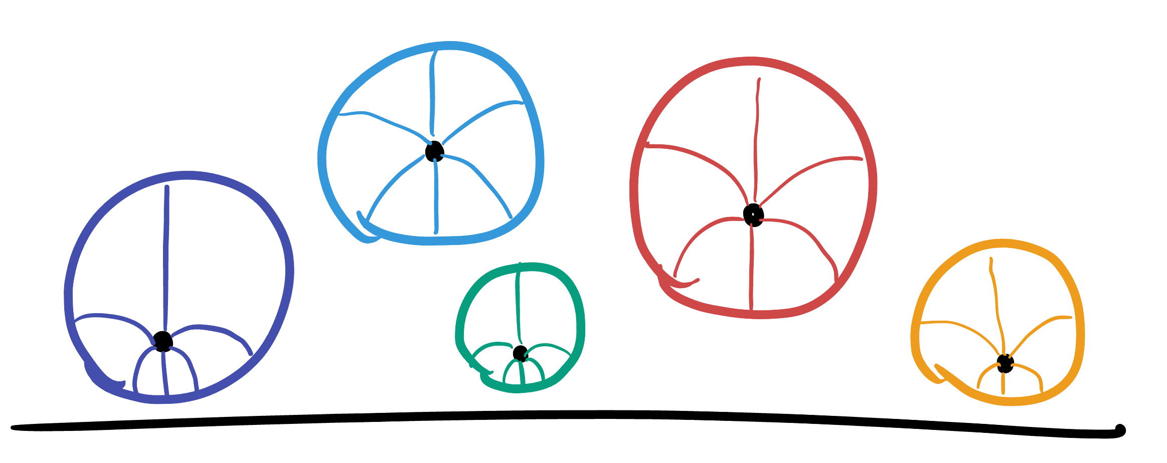
Let’s think in the Disk Model for a bit. Since space is infinitely large it seems absurd that a triangle can’t get very big! But this all has to do with the way geodesics behave. Imagining a large triangle means (in our Disk model) imagining a triangle whose three vertices are all very far away from the center, and thus appear out by the unit circle.

To form a triangle from these points, they must be connected together with geodesics. And we know what the geodesics are - they’re arcs of circles which are orthogonal to the boundary. Thus, the triangle has very skinny angles as the geodesics are almost tangent to one another. And being so skinny, these arms of the triangle can’t contain that much area.

In fact, the biggest triangle one could imagine making would have infinitely long sides, and would consist of three geodesics going all the way out to infinity.
Remark 27.2. Of course this isn’t actually a triangle as it has no vertices! Mathematicians call it an ideal triangle
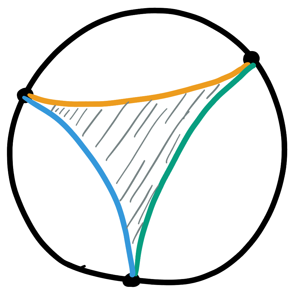
How big is an ideal triangle? To calculate, its easiest to hop over to the upper half plane. We can choose our three points so that two of them are \(\pm 1\) and the other is the projection point - off at infinity. This means our triangles geodesic sides are the unit circle, and two parallel vertical lines
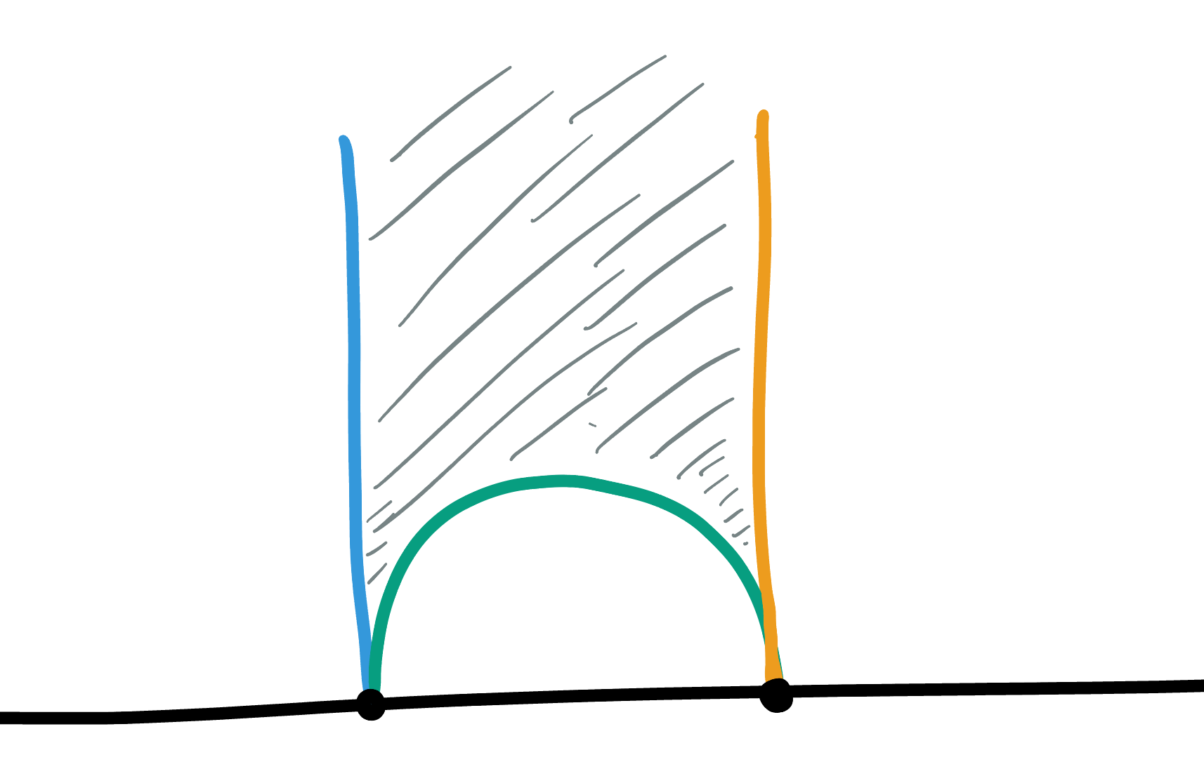
Its area is given by a double integral of \(dA\): using the scaling factor,
\[dA = \frac{dx dy}{y^2}\]
Setting up the bounds (bottom bound = unit circle, top goes to infinity) we see
\[\area = \iint_T dA = \int_{-1}^1\int_{\sqrt{1-x^2}}^\infty\frac{dydx}{y^2}\]
Doing the inner integral first:
\[\int_{\sqrt{1-x^2}}^\infty\frac{dy}{y^2}=\frac{-1}{y}\Bigg|_{\sqrt{1-x^2}}^\infty=\frac{1}{\sqrt{1-x^2}}\]
Thus, the total area is
\[\area = \int_{-1}^1\frac{1}{\sqrt{1-x^2}}dx\]
But this integral is quite familiar to us by this point in the course! Its the arc-length of the top half of the unit circle (the integral that defines arccosine).
\[\area = \pi\]
Thus we have it: all triangles in \(\HH^2\) have area less than or equal to \(\pi\), because that’s the area of the ideal triangle!