22 Examples
In this chapter we will apply some of the theory we developed to work with some well-known map projections used for depicting the earth. This is a slight digression from the logical flow of our text, as none of this work is strictly needed for anything that follows (and those interested in the purely mathematical story can move immediately to the next chapter, stereographic projection, where we apply these same techniques to the map we will use the most).
However, taking a brief look at examples serves two purposes: one, it will help us become more comfortable with the theory of maps, as we will do several explicit computations:
- We will calculate the map-length of a curve in the Orthographic projection.
- We will calculate the map-area of regions in Archimedes map, and show it is area preserving.
- We will compute angles in the Mercator map, and show it is angle preserving
And two; the study of maps is a beautiful application of mathematics to the wider human world - we might as well take a look - just for cultural reasons - while we are so nearby.
22.1 Orthographic Projection
To write down a map we need to give its chart: a map \(\phi\) from some region in \(\SS^2\) onto a region of the plane. And perhaps the simplest formula taking points in \(\EE^3\) (where the sphere lives) to points of \(\EE^2\) is just deletion of a coordinate:
\[(x,y,z)\mapsto (x,y)\]
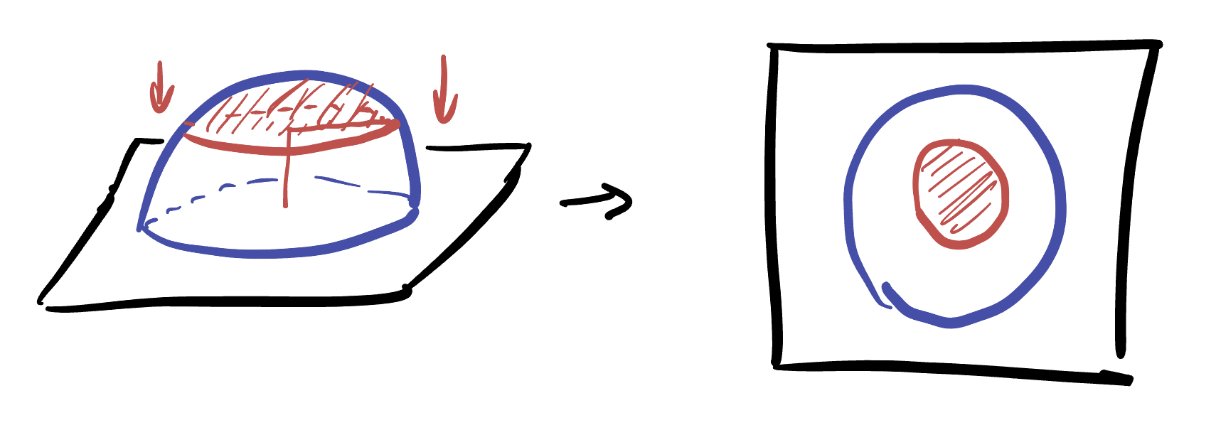
We can picture such a map as the vertical orthogonal projection of space onto the \(xy\) plane, and the result as the shadow of an object under a vertical light source
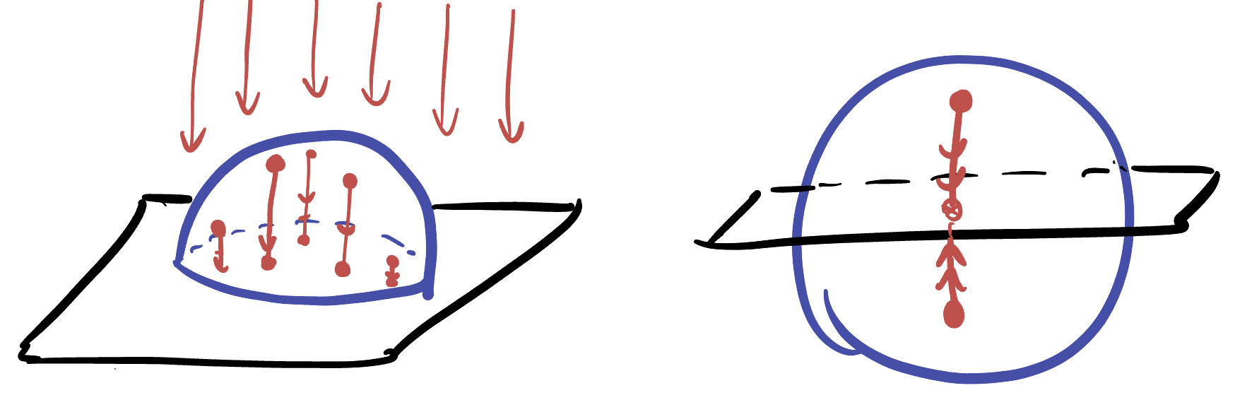
This cannot give a map of the entire earth at once, as each vertical line that intersects the sphere off the equator hits it in two points \((x,y,z)\) and \((x,y,-z)\). However, if we restrict ourselves to one hemisphere, vertical projection does define a bijection between that hemisphere and the unit disk in the plane.

Definition 22.1 (Orthographic Map) Let the region \(R\subset \SS^2\) be the northern hemisphere \(R=\{(x,y,z)\in\SS^2\mid z\geq 0\}\), and \(M\) be the unit disk in the Euclidean plane \(M=\{(x,y)\in\EE^2\mid x^2+y^2\leq 1\}\). Then the orthographic projection of \(R\) onto \(M\) is given by the chart \(\phi\) and its inverse parameterization \(\psi\), \[\phi(x,y,z)=(x,y)\] \[\psi(x,y)=\left(x,y,\sqrt{1-x^2-y^2}\right)\]

Before delving into the quantitative calculus, let’s try to develop a bit of a qualitative understanding of this map. Here’s two facts we can see directly from its definition:
- Geodesics through the north pole \(N\) on \(\SS^2\) are mapped to straight lines through the origin \(O\) in the map.
- Circles about the north pole \(N\) are sent to Euclidean circles about the origin \(O\) in the map.
To see the first point, note that (1) geodesics on the sphere are great circles, which are the intersection of \(\SS^2\) with planes through the origin. Thus (2), geodesics containing the north pole \(N\) correspond to vertical planes (containing the \(z\)-axis), and so (3) the projection of a vertical plane onto the \(xy\) plane is just a line.
To see the second point, recall that the circle of radius \(r\) about \(N\) is described a Euclidean circle in the horizontal plane \(z=\cos r\). The vertical projection deletes the \(z\) coordinate but leaves the \(x\) and \(y\) unchanged, so these circles map directly to circles in the \(xy\) plane.
This has the consequence that the equator of the sphere also maps to a circle on the plane - its the unit circle bounding our map \(M\). So, in \(M\) we have some geodesics represented by straight lines, and one geodesic represented by a circle!
Remark 22.1. This implies that other geodesics of the sphere necessarily are represented by some curves that interpolate between straight lines and circles: not all geodesics are going to look like easy-to-understand curves in our map! That’s one of the distortions we will have to learn to live with.
To get any quantitative understanding of this map, the first step is to take the derivative of the parameterization \(\psi\):
\[\psi(x,y)=\pmat{x\\y\\\sqrt{1-x^2-y^2}}\]
\[D\psi = \pmat{1&0\\0&1\\ \frac{-x}{\sqrt{1-x^2-y^2}}& \frac{-y}{\sqrt{1-x^2-y^2}}}\]
Remark 22.2. When working with such a map, its often easiest to recall that \(z=\sqrt{1-x^2-y^2}\) and just write ‘\(z\)’ anytime this expression occurs, to save mental space. Thus, we would write \[D\psi = \pmat{1&0\\0&1\\\frac{-x}{z}&\frac{-y}{z}}\]
This derivative matrix is the key to all further calculation. From it we can directly compute map-lengths of vectors and curves, map-angles, and map-areas following the general theory.
Example 22.1 (Orthographic Map-Length of \(\langle 1,0\rangle\)) If \(e_1=\langle 1,0\rangle\) is based at \(p=(x,y)\) in the orthographic map \(M\), its map-length is \[\|\langle 1,0\rangle\|_\map = \sqrt{\frac{1-y^2}{1-x^2-y^2}}\]
To see this, notice that \(D\psi_p \langle 1,0\rangle\) is simply the first column of the derivative matrix, and then we need only compute its length in \(\EE^3\):
\[\begin{align*}\left\|\left\langle 1,0,\frac{-x}{z}\right\rangle\right\|&=\sqrt{1+\frac{x^2}{z^2}}\\ &=\sqrt{\frac{z^2+x^2}{z^2}}\\ &=\sqrt{\frac{1-x^2-y^2+x^2}{1-x^2-y^2}}\\ &=\sqrt{\frac{1-y^2}{1-x^2-y^2}} \end{align*}\]
Knowing the infinitesimal lengths in the \(x\) direction lets us compute the total length of the horizontal curve \(\gamma(t)=(t,0)\) in our map. In \(M\) this is just the diameter of the disk, so its length appears to be 2: but we know this isn’t right! The diameter of the disk represents half of a great circle going from the equator to the north pole and back, so its length should be \(\pi\). Let’s do the calculation to confirm:
Exercise 22.1 The map-length of the curve \(\gamma(t)=(t,0)\) from \(t=-1\) to \(t=1\) in the orthographic projection is \(\pi\).
To see this, recall that the map length of \(\gamma\) is given by integrating the infinitesimal map-lengths of its tangent vectors: \[\len_\map(\gamma)=\int_{-1}^1\|\gamma^\prime\|_\map\,dt\]
Because \(\gamma(t)=(t,0)\) its immediate to see \(\gamma^\prime(t)=\langle 1,0\rangle\) for all time, and using the above exercise then we see at the point \((x,y)=\gamma(t)=(t,0)\), the map length of \(\langle 1,0\rangle\) is \[\sqrt{\frac{1-0^2}{1-t^2-0^2}}=\frac{1}{\sqrt{1-t^2}}\]
Integrating this gives a familiar expression: we saw this exact integral in the definition of the arc cosine function (Proposition 14.2)! Since \(\arccos(x)=\int_x^1 \frac{1}{\sqrt{1-t^2}}dt\), we see the expression we have come to is exactly \(\arccos(-1)\), which by definition is the arclength along the top half of the unit circle (ie all the way from \(x=1\) to \(x=-1\)). Thus
\[\len_\map(\gamma)=\int_{-1}^1\frac{dt}{\sqrt{1-t^2}}=\arccos(-1)=\pi\]
Beyond applying this just to the basis vector \(\langle 1,0\rangle\) we can us the same technique to find the length of any vector in \(T_pM\):
Example 22.2 (Orthographic Map Infinitesimal Lengths) If \(v=\langle a,b\rangle\) is based at \(p=(x,y)\) in the unit disk \(M\), its map-length in the orthogonal projection is \[\|v\|_\map = \sqrt{}\]
We calculate this by applyign \(D\psi_p\) to \(v\), and then finding the length in \(\EE^3\):
\[D\psi_p \langle a,b\rangle = a\pmat{1\\0\\\frac{-x}{z}}+b\pmat{0\\1\\\frac{-y}{z}}=\pmat{a\\b\\\frac{-ax-by}{z}}\]
Computing the length, we get
\[\begin{align*} \|D\psi_pv\|&=\sqrt{a^2+b^2+\frac{(-ax-by)^2}{z^2}}\\ &=\sqrt{a^2+b^2+\left(\frac{ax+by}{1-x^2-y^2}\right)^2} \end{align*}\]
Knowing the map-length of an arbitrary vector on \(T_pM\) lets us precisely describe the map-disks:
Example 22.3 (Orthographic Map Disks) At the point \(p=(x,y)\), the map-disk is the set of all vectors \(\langle a,b\rangle\in T_pM\) where \[a^2+b^2+\left(\frac{ax+by}{1-x^2-y^2}\right)^2\leq 1\]
At the center of our map where \((x,y)=(0,0)\), this equation for the map-disk reduces to the equation for the standard round unit disk \(a^2+b^2=1\). This means at the origin, we expect to see essentially no distortion in either size or angle! However, as soon as \(x\) or \(y\) are nonzero, things quickly change. Consider the point \((x,y)=(0,1/2)\). What’s the map-disk here? Just plugging in gives
\[a^2+b^2+\left(\frac{0+\frac{1}{2}b}{1-0^2-\frac{1}{4}}\right)^2\leq 1\]
and after a bit of simplification, we find
\[a^2+\frac{13}{9}b^2\leq 1\]
This is an ellipse! Thus, we see at \((0,1/2)\) the map is not distorting distance in the \(x\) direction (the coefficient of \(a\) is still 1) but it is distorting distance in the \(y\) direction.

Since it’s affecting the two directions unequally, we expect that it will not be preserving angles very well, so let’s confirm.
Example 22.4 (Orthographic Map Angle) The vectors \(\langle 1,0\rangle\) and \(\langle 0,1\rangle\) are not map-orthogonal, even though the look orthogonal in the Euclidean plane where we drew the map!
To see this, all we need to do is compute the map-dot-product between \(\langle 1,0\rangle\) and \(\langle 0,1\rangle\) and see that its nonzero. With the derivative of our parameterization already in hand, this is quick work:
\[D\psi_p\langle 1,0\rangle = \langle 1,0,-x/z\rangle\] \[D\psi_p\langle 0,1\rangle = \langle 0,1, -y/z\rangle\]
These are the two true vectors that \(\langle 1,0\rangle\) and \(\langle 0,1\rangle\) on our map represent, so the map dot product is equal to their actual dot product on \(\SS^2\):
\[\langle 1,0,-x/z\rangle\cdot \langle 0,1,-y/z\rangle = \frac{xy}{z^2}=\frac{xy}{1-x^2-y^2}\]
Thus, whenever \(x\) and \(y\) are both nonzero, the vetors \(\langle 1,0\rangle\) and \(\langle 0,1\rangle\) don’t actually point in orthogonal directions on our map!
Exercise 22.2 Can you find the coordinates \((x,y)\) of a point on the map where the vectors \(\langle 1,0\rangle\) and \(\langle 0,1\rangle\) only make a \(45\)-degree angle with one another?
Hint: can you make the problem easier for yourself by restricting \(x\) and \(y\) to lie on some line, so the problem ends up having one variable instead of two?
You can see how this would make such a map difficult to use for navigation: it would look like the map is telling you to turn \(90\) degrees but in reality you should only turn half that!
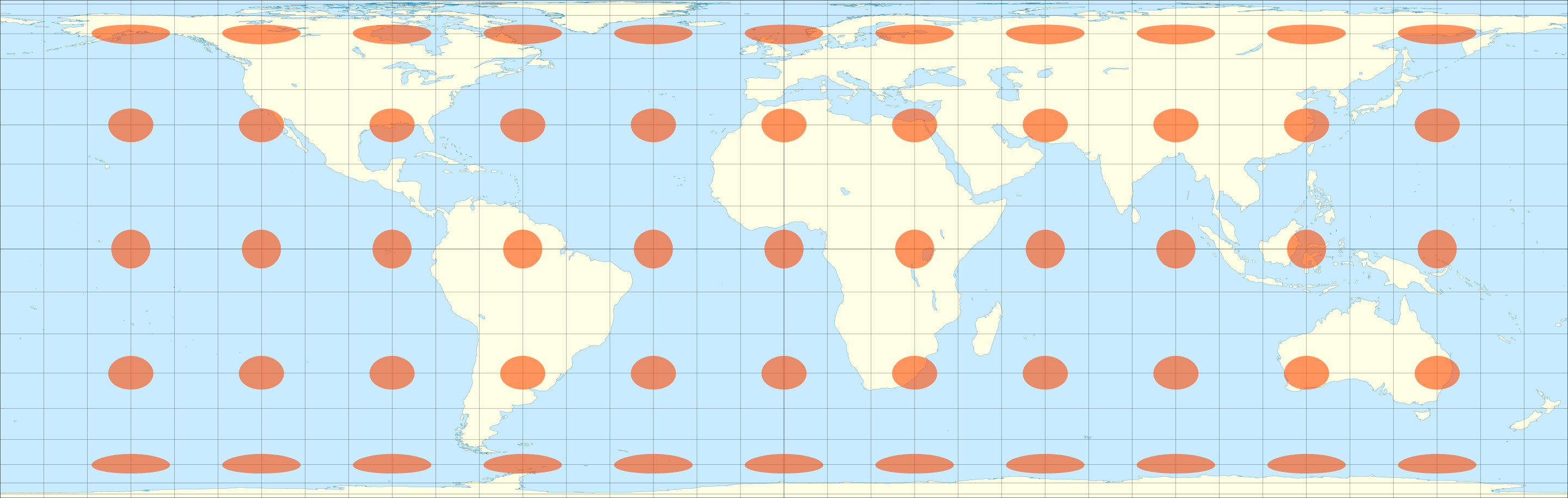
22.2 Archimedes’ Map
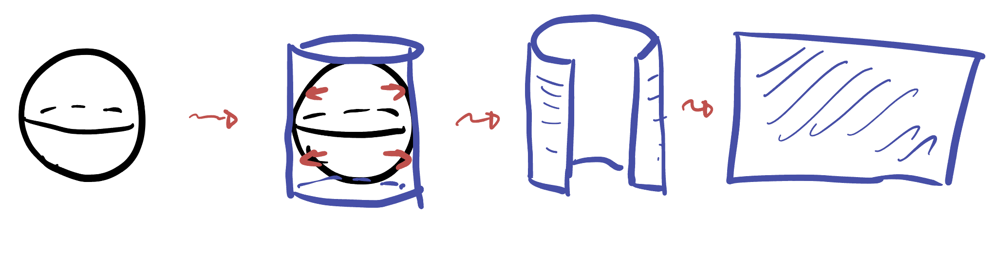
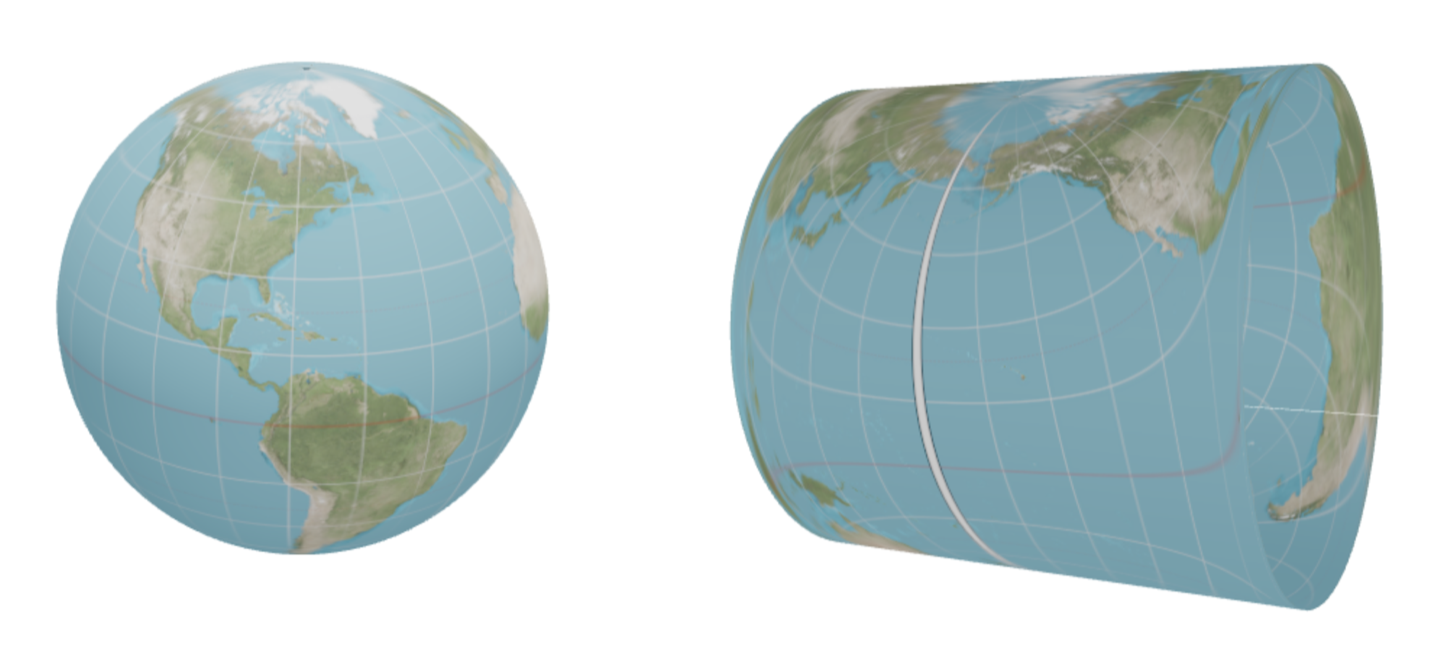
In Archimedes’ most cherished work The Sphere and the Cylinder, he proved that the surface area of the sphere and the cylinder agreed by showing that horizontally projecting the surface of the sphere onto the cylinder preserved infinitesimal areas, and thus (via integration) the total area. This suggests a means of creating a map of the earth which displays the true areas for each region: first project horizontally onto the surrounding cylinder, then unroll the cylinder onto the plane.
For step 1, what happens when we horizontally map a point \((x,y,z)\in\SS^2\) to the cylinder? Well, its height or \(z\) coordinate does not change, and the \(xy\) coordinates do not chnage direction, only length. That means that there must simply be some scalar \(s\) such that \[(x,y,z)\mapsto (sx,sy,z)\]
How do we find this scaling factor \(s\)? Well, we know at the end we want the point to lie on the cylinder, so that its \(x\) and \(y\) coordinates lie on the unit circle. This means we need
\[(sx)^2+(sy)^2=1 \,\implies\, s=\frac{1}{\sqrt{x^2+y^2}}\]
We can then use the fact that \((x,y,z)\) originally lies on the sphere, so that \(x^2+y^2+z^2=1\) to see we can replace this with \(\frac{1}{1-z^2}\) if we wish, to get
\[(x,y,z)\mapsto \left(\frac{x}{\sqrt{1-z^2}},\frac{y}{\sqrt{1-z^2}},z\right)\]
Now, we just need to unroll the cylinder onto the plane: this means we continue to leave the height, or \(z\) direction alone, but we wish to find the angle \(\theta\) which the \(x\) and \(y\) coordinates make on the unit circle. Because the tangent of this angle is opposite over adjacent, we can get an explicit formula:

\[\tan\theta = \frac{\frac{y}{\sqrt{1-z^2}}}{\frac{x}{\sqrt{1-z^2}}}=\frac{y}{x}\]
Definition 22.2 (Archimedes’ Map) Let \(R\subset \SS^2\) be everything except the north and south poles, and let \(M\subset \EE^2\) be the rectangle \(M=\{(\theta,h)\mid -\pi<\theta\leq\pi,\,-1<h<1\}\). We define Archimedes’ chart as
\[\phi(x,y,z)=(\theta,h)=\left(\arctan\frac{y}{x}, z\right)\]
and its inverse, Archimedes’ parameterization
\[\psi(\theta,h)=\left(\sqrt{1-h^2}\cos\theta,\sqrt{1-h^2}\sin\theta, h\right)\]
In cartography, this map is not named after Archimedes but rather the 17th century mapmaker Lambert, and called the Lambert Cylindrical projection, or the Lambert Equal-Area projection.


While it is natural to us earthlings to project the earth onto a cylinder whose axis passes through the north and south poles, it is by no means necessary: the sphere is homogeneous after all! So there are many unfamiliar maps that can be produced by this technique, sharing all the same mathematical properties. Here we illustrate just one option, unrolling along an axis through the equator.

To understand what Archimedes map does to regions of the sphere, a useful spot to start is to calculate its map-disks (Tissot’s Indicatrices) and see what shape they are!
Theorem 22.1 (Archimedes Map Disks) At the point \(p=(\theta,h)\) on the Archimedes map, the map disk of unit radius is given by the set of all vectors \(\langle a,b\rangle\in T_p M\) with \[a^2(1-h^2)+\frac{b^2}{1-h^2}\leq 1\]
Proof. We calculate this by just applying \(D\psi_p\) to the vector \(\langle a,b\rangle\), then finding the resulting length-squared in \(\EE^3\), and simplifying a lot.
Exercise 22.3 Do this calculation!
Because essentially all calculations require us to know infinitesimal information about the parameterization (translating vectors on the map to their true counterparts on the sphere), we begin with a calculation of \(D\psi:\)
\[D\psi = \pmat{ \partial_\theta \sqrt{1-h^2}\cos\theta &\partial_h\sqrt{1-h^2}\cos\theta\\ \partial_\theta \sqrt{1-h^2}\sin\theta &\partial_h\sqrt{1-h^2}\sin\theta\\ \partial_\theta h &\partial_h h } \]
\[=\pmat{ -\sin\theta\sqrt{1-h^2} &\frac{-h\cos\theta}{\sqrt{1-h^2}}\\ \cos\theta\sqrt{1-h^2} & \frac{-h\sin\theta}{\sqrt{1-h^2}}\\ 0&1 }\]
The map-disks are ellipses, meaning that angles in general are not preserved. However, we can calculate the area of these map-disks to understand better the area distortion (or lack thereof) on the map. The ellipses we found turn out to be lined up nicely along the two axes of \(\EE^2\), much like the ellipses whose formulas we first uncovered in Definition 13.4. Thus, their areas are computable as in Exercise 15.4: its equal to \(\pi ab\) where \(a\) and \(b\) are the ‘radii’ of the ellipse along the \(x\) and \(y\) direction.
Theorem 22.2 (Archimedes Map is Area Preserving) At every point \(p\in M\) the map-disk has area \(\pi\). Since the map disk represents the infinitesimal vector which map to the unit disk tangent to the sphere (which also has area \(\pi\)), the parameterization does not distort infinitesimal area.
Proof. If an ellipse has radii \(r_1\) along the \(x\) axis and \(r_2\) along the \(y\) axis, we saw its area is \(\pi r_1r_2\), which we could compute by stretching the unit circle in Exercise 15.4. The formula for such an ellipse is \[\frac{x^2}{r_1^2}+\frac{y^2}{r_2^2}\leq 1\] So in our case we have \(r_1=\frac{1}{\sqrt{1-h^2}}\) and \(r_2=\sqrt{1-h^2}\). These are reciprocals of one another, so \(r_1r_2=1\) and \[A=\pi r_1r_2 =\pi\] But this is the area of the unit disk! So, at each point \(p\) of the map, the mapdisks (Euclidean) area accurately represents its true area on the sphere. The map does not distort infinitesimal areas.
Because we are still learning how to compute effectively with maps, we’ll give a second proof of this fact, where we do not bother working out the details of our map disks, but rather just directly look at infinitesimal lengths are areas, figuring out what happens to an infinitesimal unit square.
Exercise 22.4 Give a second proof that Archimedes map is area-preserving, that looks at infinitesimal squares instead of ellipses. Show that at each point \(p\in M\) the vectors \(\langle 1,0\rangle\) and \(\langle 0,1\rangle\) are sent by \(\psi\) to orthogonal vectors on the sphere. Find their lengths on the sphere (ie the map-lengths), and use this data to find the area of the infinitesimal rectangle they form.
Now only does this immediately imply archimedes overall result that the two areas are equal (each area is by definition the integral of its infinitesimal areas, and we just showed all the infinitesimal areas are equal), but it also shows that the area of any region on the map accurately portrays the true area of the region it represents on the sphere.
Theorem 22.3 Let \(R\subset\SS^2\) be a region on the sphere, and \(M=\phi(R)\subset \EE^2\) its map under Archimedes chart. Then \[\area(R)=\area(M)\]
Proof. Because the chart and parameterization are inverses, we could just as well call \(\phi(R)=M\) the map, and then the original region is \(\psi(M)=R\). We compute the area of \(R\) as an integral, and use \(\psi\) to write it as an integral over \(M\):
\[\area(R)=\iint_R dA_{\SS^2}=\iint_{\psi(M)}dA_{\SS^2}= \iint_{M}dA_{\map}\]
But now we know that \(dA_{\map}=dA_{\EE^2}\), that’s what we’ve calculated! So we can sub this out, and then realize the resulting integral is just the definition of the Euclidean area of \(M\) in the plane:
\[=\iint_M dA_{\EE^2}=\area(M)\]
However, its important not to forget what we learned along the way: the map-disks for Archimedes map form extremely distorted ellipses as one approaches the poles: with horizontal length stretching near infinite and vertical height crushing to zero. This map massively distorts the shapes of regions, distances between points and angles between curves in its attempt to preserve area. Like the orthographic map before it, this makes Archimedes’ map unsuitable for navigational tasks, where figuring out accurately what direction you must go to reach your desired destination is of utmost importance.
22.3 Equirectangular Projection
There is an entire collection of maps which are defined as modifications of Archimedes’ original idea, these days called cylindrical projections as they start by projecting onto a cylinder. Perhaps the two most common of these are the Mercator projection (discussed in the next chapter as a potential final project opportunity), and the Equirectangular projection, which I will only briefly mention here (for anyone who is doing a final project on Maps and would like another, easy-to-compute-with and yet still real-world example).
The problem the Equirectangular projection tries to solve is the vertical distortion of Archimedes’ map. Archimedes made the vertical height on the map equal the vertical height of the sphere at that point: this clever move ensured area was preserved, but what if we wanted the vertical height on the map to actually be related to the north-south distance? Archimedes’ map fails badly at this, as we see in the picture above.
What we want from our new map projection is that it
- Continues to be a cylindrical projection
- Distance along the (vertical) \(h\) axis of the map accurately reflects the actual geodesic distance along lines of longitude on the sphere.
Because we are still projecting onto a cylinder, the chart for such a map is still going to have \(\theta=\arctan(y/x)\). But as arclength is angle, the height (distance from the equator) will need to be the angle \(\varphi\) that a point on the sphere makes with the \(xy\) plane:
Definition 22.3 The chart for the equirectangular projection is defined on the region \(R\subset\SS^2\) of the sphere containing all points except the north and south poles, and maps onto the rectangle \[M=\{(\theta,\varphi)\in\EE^2\mid -\pi\leq \theta\leq\pi,\,\, -\pi/2\leq \varphi\leq \pi/2\}\]
by the chart function
\[\phi(x,y,z)=\left(\arctan\frac{y}{x},\arcsin z\right)\]
Exercise 22.5 Derive the parameterization for the Equirectangular projection.


Exercise 22.6 Spherical coordinates in mathematics and physics are almost the same as the equirectangular projection: the only difference being a convention on where to measure the angle \(\varphi\) from. Here we’ve measured it from the equator, so that it accurately captures latitude on the earth. But in spherical coordinates it is usually measured from the north pole.
Write down the chart and parameterization for spherical coordinates, and see that it is what you are taught in multivariable calculus!
Because this map captures distance accurately along the equator, as well as north-south distance along lines of longitude, it is an easy map to work with, and has become the default map in many contexts.
Exercise 22.7 Find the important map-quantities in the equirectangular projection:
- Find the map-length of a vector \(v=\langle a,b\rangle\) based at \((\theta,\varphi)\in M\).
- Find the equation for the map-disk at \((\theta,\varphi)\). Show that it’s an ellipse: what do its vertical radius and horizontal radius tell you about the map?
- Does this map preserve angle?
- Find the map-area: since horizontal and vertical lines in \(M\) map to orthogonal curves on \(\SS^2\) (latitude and longitude), infinitesimal squares on \(M\) are taken to infinitesimal rectangles on \(\SS^2\). Does this map preserve area?
