26 Models
At this point we have a lot of ideas of what negatively curved, or hyperbolic space is like, but we do not have a concrete way to work with it. This causes two major problems:
We don’t have any means of discovering new facts about hyperbolic space everything we’ve learned as come from our understanding of spherical geometry, passed along the transition as curvature goes to \(-1\). This is a great approach for learning facts about hyperbolic geometry that are analogous to the sphere, but it leaves us blind to any potential differences. And we know there will be differences! As a concrete case where this will be important: we know on the sphere there’s just one type of (orientation preserving) isometry: rotations. But in the Euclidean plane there are two types: translations and rotations! How many types of isometries does hyperbolic space have?
How do we really know that hyperbolic space even exists? For both the Euclidean plane and the sphere, we started with a definition we specified the points of the geometry, its tangent vectors, and its infinitesimal length / inner product. Then we built up all other results as theorems. But so far we have no analogous construction of hyperbolic space. We have a bunch of theorems about how distance should work, or area should work, but we don’t even have a clear notion of what the points are we are measuring distance between! Because the implications of this discovery are enormous (namely, it resolves the most important problem of the greeks, which was open for more than two thousand years), we should not be satisfied with this state of affairs. Its like the discovery of a new species deep in the jungle: its useful to have a detailed description of the creature, but this isn’t enough. If you claim to have discovered Bigfoot, you’d better present a specimen!
In this chapter we aim to simultaneously remedy these two concerns, and produce an explicit model of hyperbolic space.
26.1 Conceptual Troubles
Upon sitting down to try and rigorously define the hyperbolic geometry we’ve glimpsed through the transition, we immediately hit a conceptual hurdle: how are we supposed to find the right set of points and definition of infinitesimal length? For both the Euclidean plane and the sphere, we didn’t have to confront this problem because we essentially already knew the right definitions to write down: we’ve all seen many planes and spheres before in daily life. But negatively curved space? We do see around us spaces that have some negative curvature, like a Pringle chip
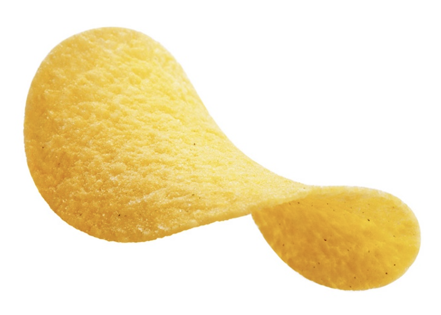

But this is not hyperbolic space. The curvature of a pringle chip is more negative at the center and less negative (closer to flat) the farther out you go: here’s a zoomed out view of the pringle chip function \(x^2+y^2\)
But hyperbolic geometry is supposed to have curvature \(-1\) everywhere: indeed, if we really reach this space along a path including spheres and the Euclidean plane, it should be both homogeneous and isotropic. A pringle chip is neither! Other shapes familiar from the world around us are closer to having constant negative curvature, such as the surface of a kale leaf, certain types of coral, or the wavy back of a nudibranch.


Anytime evolution tries to increase the area of something beyond Euclidean constraints, it resorts to negative curvature.
However these surfaces are all rather small: hyperbolic space is supposed to be infinite! And its not quite clear upon looking at one of these surfaces how to continue it, and make it bigger. As the surface grows exponentially fast it wrinkles more and more - it seems hard to believe one could continue this infinitely without the surface self-intersecting, or worse - having a crease or points of non-differentiability (rendering all of our calculus based tools useless).
In fact, this is a very reasonable worry to have. This was though deeply about at the turn of the 20th century, and it was actually proved that there is no way to do this.
Theorem 26.1 (Hilbert’s Theorem) There is no surface in \(\EE^3\) which has the geometry of the hyperbolic plane.
Remark 26.1. In the technical statement of the theorem, it is important that the surface is described by at least second differentiable functions for the proof to go through. But this is no serious restriction as we are already working in a world where calculus forms the foundations of everything we do, and you need second derivatives to even define curvature (meaning, if our surface were not described by such functions, then the limit defining curvature would not exist at some points).
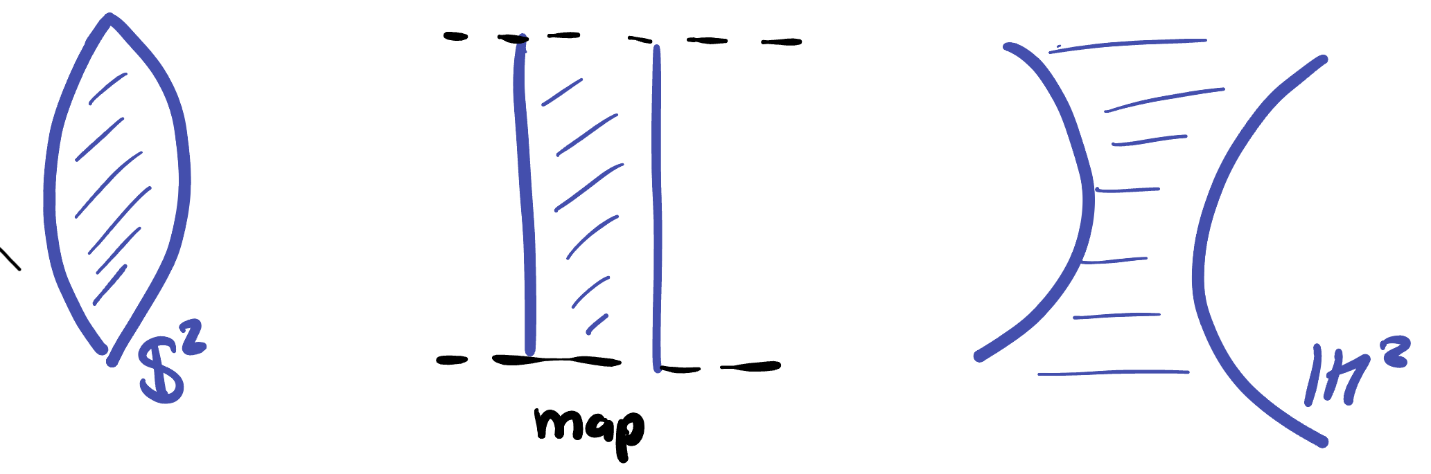
Thus, we must abandon hope of being able to work exactly as we did for the sphere, where we found a subset \(\SS^2\subset\EE^3\) of points, found the tangent spaces, and then defined all geometry using the euclidean dot product on these tangent spaces. Instead, we are going to have to make use of our study of maps, and the flexibility they provide.
26.2 Making a Map
So, there is no surface in \(\EE^3\) which has the same geometry as the hyperbolic plane. But that’s alright - there isn’t any region in \(\EE^2\) that has the same geometry as \(\SS^2\) (via The Mapmaker’s Dilemma) but we are able to completely accurately do computations about \(\SS^2\) using regions of \(\EE^2\) via a map.
In the previous part, our construction of a map went like this: we started with the ‘actual’ sphere, and wrote down a chart onto a region of the plane, and its inverse, a parameterization \(\psi\) taking that region to the sphere. We then used this parameterization \(\psi\) to make all geometric properties of the sphere computable on the map directly (map-lengths, map-angles, map-dot-products, map-areas, etc). At the end of this procedure, we are left with a region on the plane, and a new rule on how to compute geometric quantities in that region (different from the original Euclidean way). But, if we follow these new map-formulas correctly, it is precisely as good as if we worked directly on the sphere itself.
Taking this observation to its logical (but shocking) conclusion was the subject of Riemann’s Habilitationsschrift, or post-doctorate research assigned by Gauss. Riemann realized that to do geometry, maps are all you need!
The Fundamental Insight of Riemannian Geometry: Any region of the plane, together with a rule for how to perform the dot product at each point (and thus, to compute infinitesimal lengths and angles) is a map of some geometry - just perhaps a geometry that we have never before seen.
Example 26.1 From Riemann’s perspective, if I were to write down the strip in the plane \(|y|<\pi\) and explain that at the point \((x,y)\) in this strip, the dot product of two vectors \(v=\langle,v_1,v_2\rangle\) and \(w=\langle w_1,w_2\rangle\) is
\[\frac{v_1w_2+v_2w_2}{\cosh^2 y}\]
Then I am describing a true geometry. No matter what questions you asked me about the geometry, with enough work I’d be able to do the calculations and answer them, so this is truly indistinguishable from having the ‘real thing’ in front of me - whatever that might mean! Indeed - Riemann’s whole point is that there is no real thing above and beyond the map: the map is just as real as anything else!
Of course in this particular case if I sat down and started doing lots of calculations, I would realize that this geometry has some familiar properties: all of its geodesics have length \(2\pi\), triangles angles are determined by their angle sum, and so on. This is just the dot product that we found for the Mercator projection of the sphere!
But Riemann’s genius is to go further, and take something like the below seriously
\[\frac{v_1w_2+v_2w_2}{\cos^2 y}\]
or even
\[(x^2+1)v_1w_1+e^{x+\sin y}v_2w_2\]
These dot products describe some geometric spaces we have not yet encountered. And its up to us to do math, and figure it out!
In taking this bold step, Riemann reduced the set of things needed to do geometry down to one: just a dot product on a region in the plane, or a region in some higher dimensional (euclidean) space. Because this dot product is the main tool we use to find infinitesimal lengths, then lengths, then distances (and hence produce a metric), it’s called the Riemannian metric.
Definition 26.1 (Riemannian Metric) Given a region \(R\subset \EE^2\) in the plane, a Riemannian metric on \(R\) is a choice of formula for the dot product at each point \((x,y)\in R\). Any such choice is specified by three functions, \(G(x,y)\), \(E(x,y)\) and \(F(x,y)\) where we write
\[(v\cdot w)_{(x,y)} = G(x,y)v_1w_1+ F(x,y)(v_1w_2+v_2w_1)+F(x,y)v_2w_2\]
Remark 26.2. The two middle terms both have the same coefficient \(F(x,y)\) because the order we take the dot product in shouldn’t matter: we want \(v\cdot w = w\cdot v\).
Thus, as we move around to different points \((x,y)\) the definition of the dot product is allowed to vary, representing that our map might be distorting the underlying geometry by different amounts at different points.
Exercise 26.1 Write the Riemannian metric (as a matrix) for the stereographic and mercator projections of the sphere.
Remark 26.3. Riemann actually went further than this: recalling that it is not even possible to cover the entire earth wtih a single chart, it would be shortsighted to define geometry in general in terms of a single map. Instead, a space is called a manifold if there is some atlas of charts covering it, and a Riemannian manifold if each of these charts has a Riemannian metric.
Alright, so how do we go about finding a map, or in mathematical terminology, a Riemannian metric for hyperbolic space? We continue pushing spherical things beyond infinity, of course! We can take any map we like for the sphere and run our hyperbolization procedure on it: write it for radius \(R\), convert to curvature, then push to \(\kappa=-1\).
Because out of all the maps we studied stereographic projection certainly had the (mathematically) nicest properties, we will start wtih this. We found the dot product for a sphere of radius \(R\) to be, at the point \(p=(x,y)\)
\[ (v\cdot w)_\map=\frac{4R^4}{(R^2+|p|^2)^2}(v\cdot w)_{\EE^2}\]
Writing this in terms of curvature is straightforward, as only even powers of \(R\) show up already
\[\begin{align}(v\cdot w)_\map &=\frac{4\frac{1}{\kappa^2}}{(\frac{1}{\kappa}^2+|p|^2)^2}(v\cdot w)_{\EE^2}\\ &=\frac{4}{\kappa^2(\frac{1}{\kappa}+|p|^2)^2}(v\cdot w)_{\EE^2}\\ &=\frac{4}{(\frac{\kappa}{\kappa}+\kappa|p|^2)^2}(v\cdot w)_{\EE^2}\\ &=\frac{4}{\left(1+\kappa|p|^2\right)^2}(v\cdot w)_{\EE^2} \end{align}\]
This formula is exactly equivalent to what we already knew for the sphere when \(\kappa>0\), but continues to make sense when \(\kappa\leq 0\). In the case that \(\kappa\) is negative, its easiest to write things in terms of \(|\kappa|\) as usual, where we get
\[(v\cdot w)_\map=\frac{4}{\left(1-|\kappa||p|^2\right)^2}(v\cdot w)_{\EE^2}\]
This map has some interesting behavior! Its not defined on the whole plane, but only on a subset of it: once \(|p|\) reaches a size of \(1/\sqrt{|\kappa|}\) then we get division by zero. In particular, for the “unit sized” space \(\kappa=-1\) the map is only defined inside the unit disk! Nonetheless as we will shortly seen, the geometry described by this map is infinite. This is the so-called disk model of the hyperbolic plane.
26.3 The Disk Model
Definition 26.2 (Disk Model of \(\HH^2\)) The disk model (also called the Poincare Disk or the Beltrami-Poincare Disk) is given by the unit disk in the plane \[\{(x,y)\in\EE^2\mid x^2+y^2<1\}\] together with the Riemannian metric \[(v\cdot w)_{PD}=\frac{4}{(1-|p|^2)^2}(v_1w_1+v_2w_2)\]

What does this model of the hyperbolic plane look like? Well, we see immediately that it is conformal (no surprise, since stereographic projection was as well) since the dot product is a multiple of its Euclidean counterpart. Thus, any angles we see in the disk will represent the true angles on the plane. But the scaling factor has completely the opposite behavior of stereographic projection. It approaches infinity as we head towards the boundary of the disk, which means that objects there are much bigger than they appear. Equivalently, if you move an object towards the boundary of the disk it should appear to shrink in size!
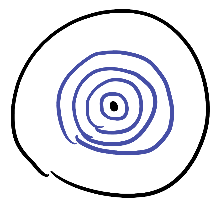
These strange distortions of size aside, there are many positive qualities about this model. In some ways, having built our model of hyperbolic space inside of the Euclidean plane is actually more useful than doing something else - as we can use things we know about \(\EE^2\) to help us deduce facts about \(\HH^2\): here’s a useful example, with almost no knowledge we can deduce the circles in \(\HH^2\) about the center of the disk model.
First, Euclidean rotations of the plane about the origin restrict to isometries of the Disk Model of \(\HH^2\): Rotation isometries of the plane do not change the distance of a point from the origin, and they do not affect the Euclidean dot product of two tangent vectors. Because the hyperbolic disk dot product is just the Euclidean one rescaled by a function of distance from the origin, it is also unchanged by a rotation, so these rotations are hyperbolic isometries!
Knowing this, we can see that hyperbolic circles about the origin of the disk model are Euclidean circles. Euclidean rotations of \(\HH^2\) about the origin are isometries of the model, so every point on the same Euclidean circle as \(p\) about \(O\) is the same hyperbolic distance from \(O\): this is the definition of a hyperbolic circle!
Note that this argument does not actually tell us the hyperbolic radius of this circle, because we don’t yet know how to measure the hyperbolic distance in our model from \(O\) to \(p\). We will figure out how to do this in the next chapter, and confirm this space really does have curvature \(-1\).
The disk model is wonderful for depciting the hyperbolic plane, and for doing any sort of calculations that involve rotational symmetry, as we saw above. But serveral other computations are rather challenging in the disk model, due to the fact that the scaling factor in front of the dot product depends on the *euclidean distance from \(O\). This makes some work with \(x\) and \(y\) coordinates cumbersome, as they naturally describe affine lines and not circles in the plane.
But there is nothing tying us down to exclusively use this disk we just discovered! Its just one map, after all. And, just like for the sphere, different maps are best suited for different purposes. In the next section below we derive the map perhaps most used for computations, the Half Plane Model.
26.4 The Half Plane Model
The half plane, or upper half plane, or Poincare half plane model of the hyperbolic plane is so named becasue it is a map which is drawn on the upper half space of the Euclidean plane. In fact this upper half plane map is just a different perspective on the map we already drew above, using stereographic projection!
We saw previously that stereographic projection lets us write down a conformal map that takes the unit disk to the half plane by projecting to the sphere, rotating, and re-projecting to the plane:

Indeed, in Exercise 60 you actually derived the formula expressing this map, which after a little simplification is
\[\phi(x,y)=\left(\frac{2x}{x^2+(y-1)^2},\frac{1-(x^2+y^2)}{x^2+(y-1)^2}\right)\]
We can similarly derive its inverse (let’s call it \(\psi\)), which maps the upper half plane to the disk.
\[\psi(x,y)=\left(\frac{x^2+y^2-1}{x^2+(y+1)^2},\frac{-2x}{x^2+(y+1)^2}\right)\]
Remark 26.4. These maps can be described much shorter using complex arithmetic: if we write \(z=x+iy\) for a point in the plane, then \[\phi(z)=i\frac{1+z}{1-z}\] and its inverse \(\psi\) is \[\psi(z)=\frac{z-i}{z+i}\]
We now use this to transfer the disk model itself onto the upper half plane. The result is going to be a conformal model of Hyperbolic space as well (the original model was conformal, and this new model is the result of applying a conformal map to it), so we know the dot product is just going to be some mutliple of the Euclidean version. And all that needs to be done is calculate that scaling factor!
Exercise 26.2 (The Scaling factor of the UHP) At a point \((x,y)\), show that the scaling factor for the dot product is simply \(\frac{1}{y^2}\), following the steps below:
- Start with a unit vector, say \(\langle 1,0\rangle\) based at some point \((x,y)\) in the upper half plane.
- Apply \(D\psi\) to this vector, to move it to the disk model, based at the point \(\psi(x,y)\).
- Find the scaling vactor at this point, and simplify the result!
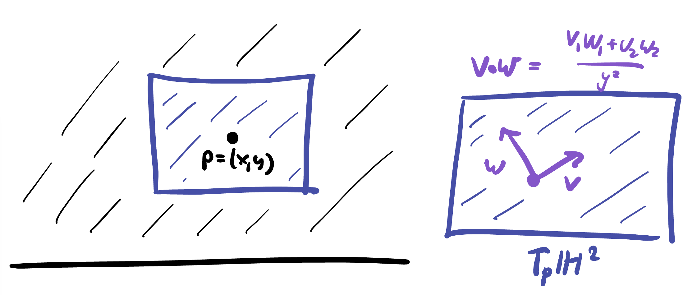
Definition 26.3 (Half Plane Model of \(\HH^2\)) The points of the half plane model of hyperbolic space are \[\{(x,y)\mid y>0\}\] together with the Riemannian metric \[(v\cdot w)_{HP}=\frac{v_1w_1+v_2w_2}{y^2}\]
Thinking again about what this map represents, we know that since its conformal we can trust the angles we see to be accurate, but we should distrust lengths. Since the scaling factor is going to infinity as we approach the \(x\)-axis, we know that the true size of a shape is much larger than it appears down by the axis. This is analogous to the what happens near the unit circle in the disk model.
As \(y\to\infty\) the scaling factor approaches zero, which says that the half plane model also distorts distances the other way as we move up, away from the line \(y=1\) where infinitesimal distances are correct. Objects high up in the half plane appear much larger than they actually are, like Greenland on the Mercator map of the sphere.
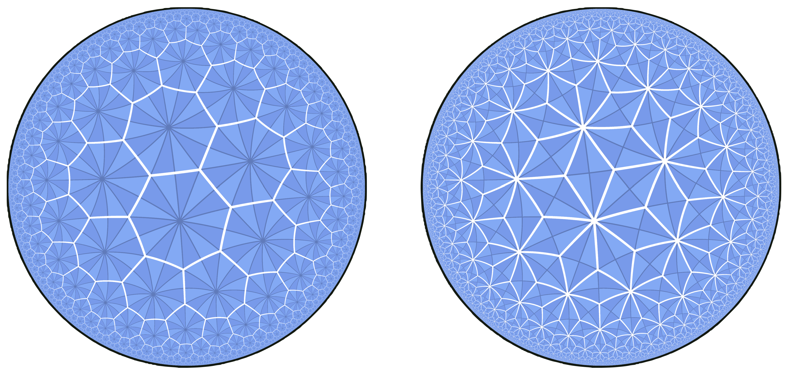
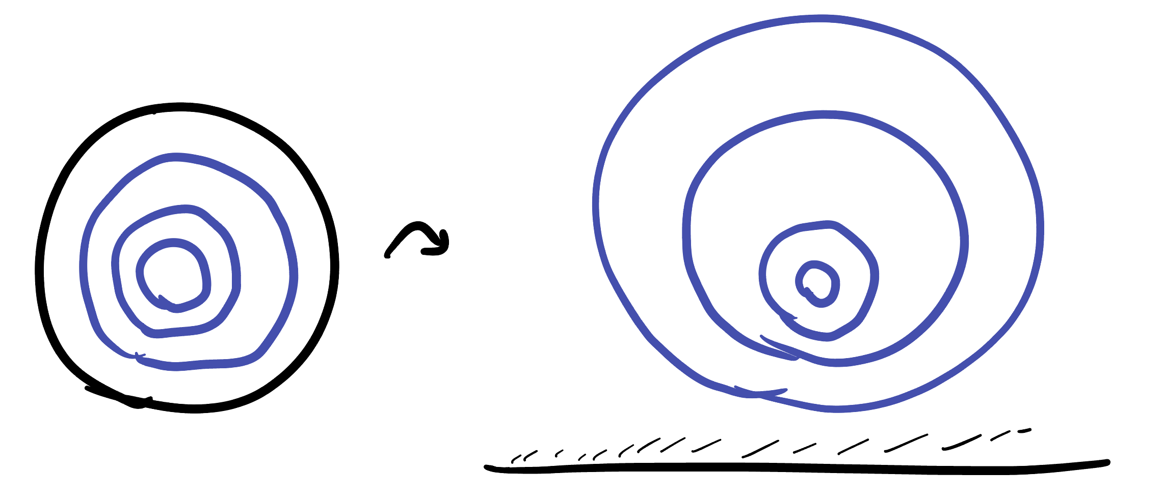
It will prove very useful to us to be able to go back and forth between the disk and half plane models of hyperbolic space. Pre-empting this, we had a homework exercise to think through this map when it was first derived (just in the context of stereographic projection), which we will now go through together. Say we start with this grid of polar coordinates in the disk:

When we map to the upper half plane, we know a couple things: - By direct calculation, we can find the origin \(O\) maps to \((0,1)\). - The map sends generalized circles to generalized circles, so circles about \(O\) go to generalized circles.
- But, a circle only maps to a line if it passes through the projection point. None of these do - they’re all inside the lower hemisphere, and then rotated to be inside the rightmost hemisphere, and the projection point is the north pole. Thus, they project to circles:
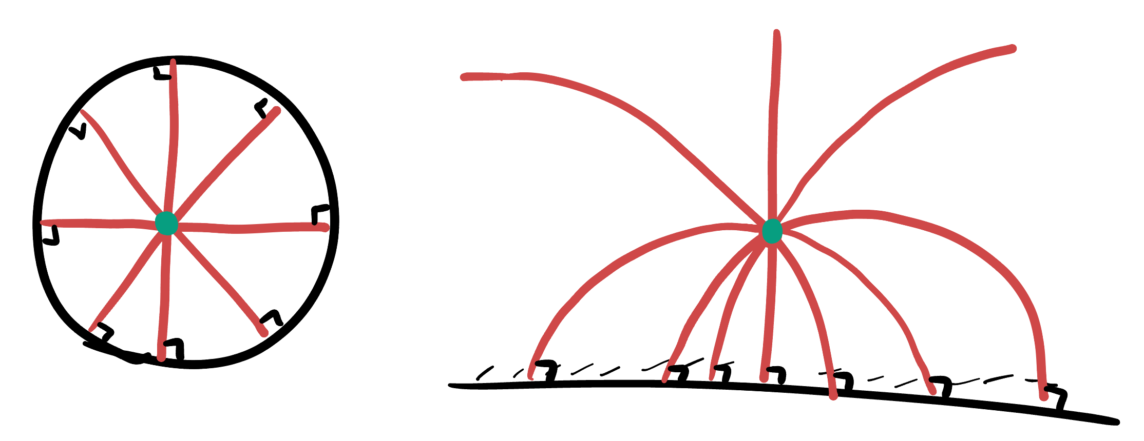
- Similarly for the lines through the origin - these go to generalized circles.
- The map is conformal, so it preserves angles. The two original families of curves intersected orthogonally, so the new curves must as well.
- In particular, the radial lines that intersected the unit circle orthogonally now intersect the \(x\)-axis orthogonally.
This tells us that the radial lines must go to lines/segments of circles passing through \((0,1)\) and hitting the \(x\) axis orthogonally. The only line with both these properties is the \(y\) axis, so the rest must be half-circles, whose centers are on the real axis
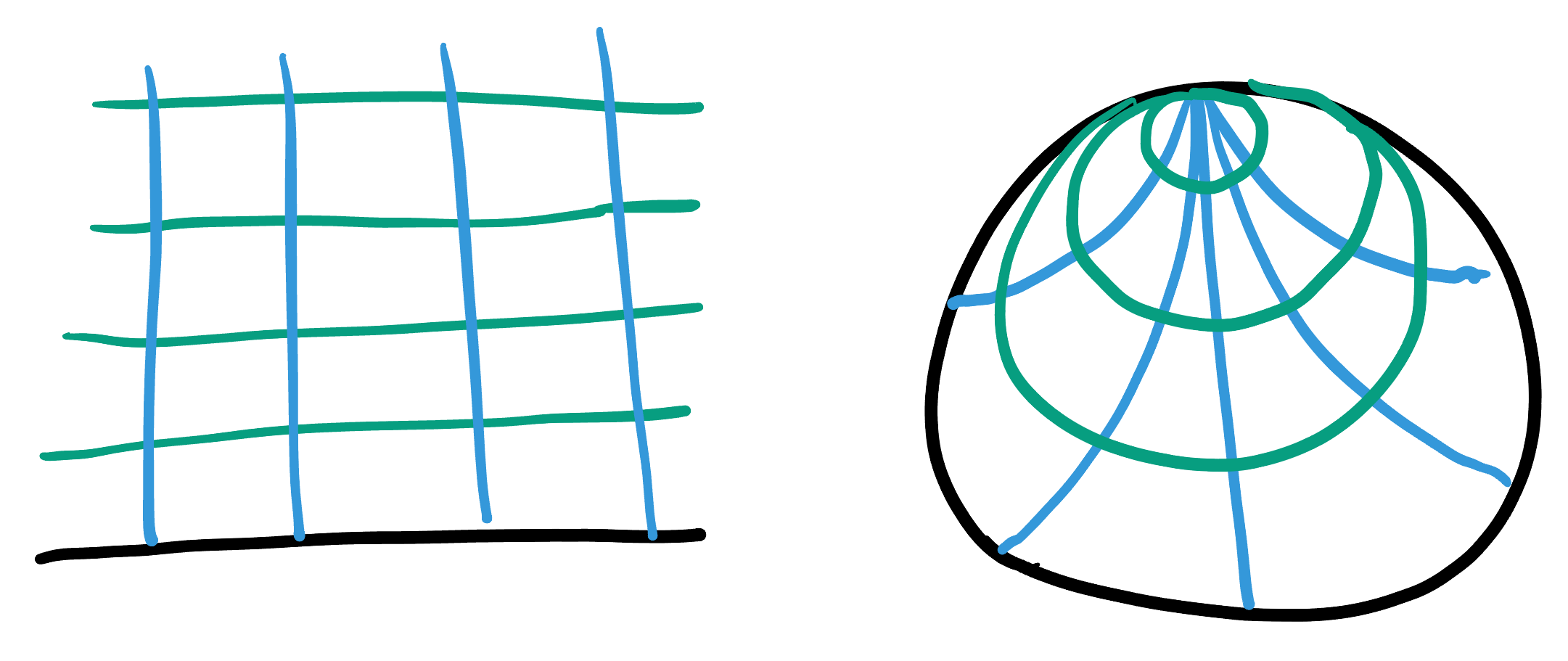
We can run a similar argument in reverse, to think about what the standard \(xy\) grid pattern on the half plane would look like in the disk. Here we find that both families of curves must go to arcs of circles in the disk, like below:
26.5 Other Maps
We discoverd the disk model, and later the half plane model starting with the stereographic projection map. And this was a good choice - the niceness of stereographic projection led to two particularly nice maps of hyperbolic space! But these are far from the only maps: its possible to apply this same procedure to many maps of the sphere, and arrive at a map of hyperbolic space.
26.5.1 Mercator
What happens if we take the Mercator projection and extrapolate to negative curvature? The Mercator projection’s dot product is also conformal and given by a relatively simple formula:
One may (correctly) guess the form this will take if we were to (1) write it out for a sphere of radius \(R\) (2) convert this to curvature (3) push the curvature to a negative number, using the taylor series representation and (4) convert back to trigonometric form at \(\kappa = -1\): it will switch the denominator \(\cosh(y)^2\) for simply \(\cos(y)^2\)!
Exercise 26.3 Check this.
The result is a map onto the plane of geometry with curvature \(-1\): hyperbolic geometry! This map’s dot product is
\[(v\cdot w)_{(x,y)}=\frac{v_1w_1+v_2w_2}{\cos^2 y}\]
Which becomes undefined when \(\cos y=0\), so the region where the map makes sense around the origin is in the strip \[\left\{(x,y): |y|<\frac{\pi}{2}\right\}\]
The dot product on this strip has scaling factor diverging to infinity towards its boundary. This tells us we should expect that objects appear very small near the boundary of the strip, compared to their actual size.

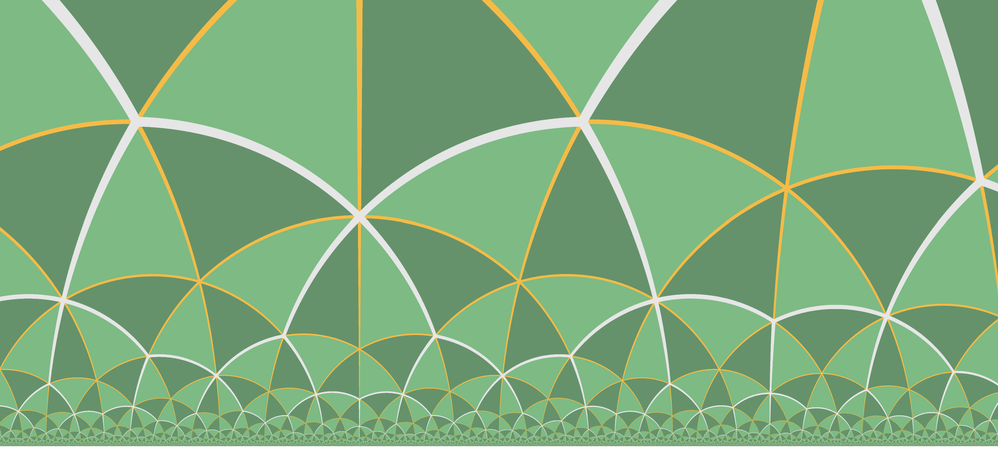
This is often called the band model, as it is defined in the interior of a band, or horizontal strip in the Euclidean plane. You may recognize the band model from our book’s front cover!
Exercise 26.4 Which isometries are easy to see must exist in the band model?
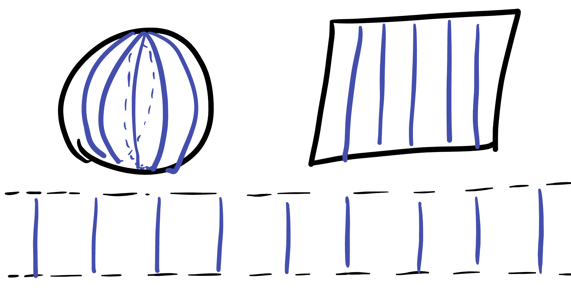
While we will wait until the next chapter for formal verification, we can already figure out what some of the geodesics in the band model must be. In the Mercator porjection, the equator geodesic was represented by the line \(y=0\) in all curvatures - and so once the curvature becomes negative this line is still a geodesic of our model! Other parallel lines to it on the sphere wer not geodesics (they were lines of latitude, or circles around the poles), and this also remains true in the Band model.
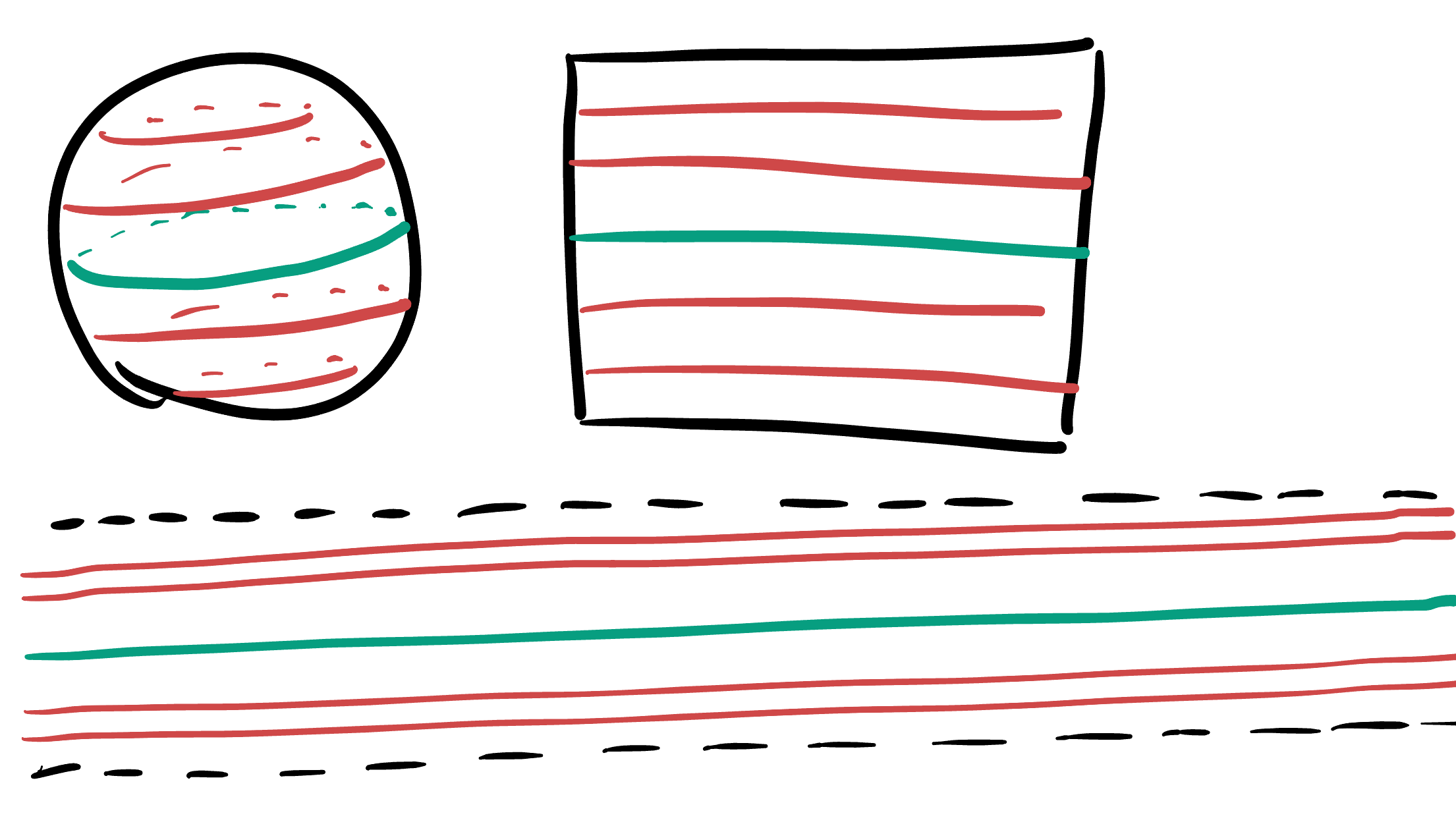
Vertical lines in the Mercator projection are lines of longitude, which are geodesics for spheres of every curvature. Thus, passing to negative curvature we find that all vertical lines in the Band model still to be geodesics:
Its useful to pause here and think about what a vertical strip between two such curves on our map actually represents. On the sphere, the scaling factor \(1/\cosh(y)\) shrank towards zero as we moved away from the equator, meaning that the lines were actually closer than they appear.
But once \(\kappa=-1\) and the scaling factor becomes \(1/\cos(y)\) which gets extremely large as \(y\) grows, meaning that these geodesics actually become much farther apart than they appear to be. Quantitatively: the distance along a horizontal line is \(1/\cos(y)\) times as long as it appears! This is the first quantitative measurement where we can confirm that geodesics indeed race away from one another in negative curvature.
Remark 26.5. Note this isn’t precisely the distance between points, as we are measuring the length of a horizontal curve which is not a geodesic. To find distance we’ll have to do some more computations in the next chapter.
26.5.2 Archimedes?
Archimedes map of the earth was an equal area projection. So far, all of our maps of hyperbolic space have been conformal but have massively distorted area. Can you find an analog of Archimedes map in negative curvature, to give an area-preserving option?