23 Mercator
The Mercator projection is the classic map
One means of building Mercator’s map is to begin with Archimedes’, and and perform some modifications. We will follow this, and will attempt to change as little from the previous map as possible: indeed we will attempt to construct this new map also by first projecting the sphere onto its bounding cylinder, and then unrolling that cylinder onto the plane.

The only choice we made in the above derivation of Archimedes’s map was that the projection was horizontal, or that the height \(h\) on the map was equal to the original \(z\) coordinate. Here, we must do something else (lest we end up with the same map!) so we let \(h\) be a function of \(z\): this is equivalent to first doing Archimedes map, then stretching the vertical axis of the cylinder by a function \(H\). Different choices of \(H(z)\) will describe different cylindrical projections, and our goal here is to find a good choice for \(H\).
Definition 23.1 (A General Cylindrical Projection) Let \(H(z)\) be any height function taking the latitudes of the unit sphere \(z\in[-1,1]\) to some height \(h\) along the cylinder. Then the cylindrical projection corresponding to \(H\) is given by \[(x,y,z)\mapsto \left(\frac{x}{1-x^2-y^2},\frac{y}{1-x^2-y^2},H(z)\right)\]
There are all sorts of maps you can make by choosing different functions \(H\) here (and then unrolling the resulting cylinder onto the plane). But most of them will distort angles: they’ll take infinitesimal squares on the map to infinitesimal rectangles on the sphere, and vice versa (like Archimedes’ example). Only one will take squares to squares at every single point - and this is what Mercator was after!
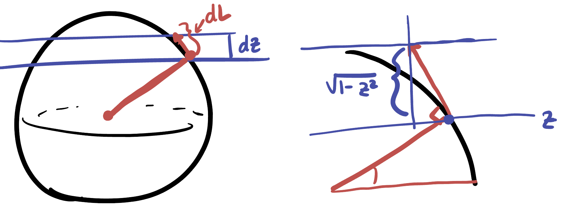
Here was his idea: we know how much the circle starting at height \(z\) has to get stretched horizontally - because we are projecting it onto the cylinder of radius \(1\). At height \(z\), the radius of the circular slice of the sphere \(x^2+y^2+z^2=1\) must be
\[r=\sqrt{x^2+y^2}=\sqrt{1-z^2}\]
Thus its circumference is \(2\pi\sqrt{1-z^2}\), and it is going to get stretched to the unit circle, with circumference \(2\pi\). So, we know that our map is scaling by a factor of \(\frac{1}{\sqrt{1-z^2}}\) horizontally. This means that vertically, we must ensure it is also scaling by \(\frac{1}{\sqrt{1-z^2}}\)!
But the vertical direction involves two stretches: first we need to think about the effect of horizontal projection onto the cylinder, and then second, we need to tack on the vertical stretch induced by \(H\).
The first of these is something we can already compute using our knowledge of Archimedes map! At a point \(p\) on Archimedes’ map, the vertical vector \(\langle 0,1\rangle\) points along this cylinder. Its map-length is
\[\|\langle 0,1\rangle\|_\map =\|D\psi_p\langle 0,1\rangle\|_{\SS^2}=\left\|\pmat{\frac{-h\cos\theta}{\sqrt{1-h^2}}\\\frac{-h\sin\theta}{\sqrt{1-h^2}}\\ 1}\right\|_{\SS^2}\]
Where we found the vector as the second column of \(D\psi\) for Archimedes map. Computing this length with the 3D pythagorean theorem (which measures the true length on the sphere, as the tangent spaces to \(\SS^2\) use the Euclidean dot product), we see
\[\|\langle 0,1\rangle\|_\map = \sqrt{1+\frac{h^2}{1-h^2}}=\frac{1}{\sqrt{1-h^2}}\]
This means a vector of Euclidean Length 1 on the map gets sent to a vector of length \(1/\sqrt{1-h^2}\) on the sphere, so when going from the map to the sphere the length of a vector is divided by \(\sqrt{1-h^2}\). This means inversely, projecting from the sphere to the map multiplies the true length of a vector by \(\sqrt{1-z^2}\) (where we use \(z\) on the sphere and \(h\) on the plane/cylinder, just to keep things separate).
Exercise 23.1 Check all this!
Now we’re ready to think about the stretch \(H\) we need. Going from the sphere to the cylinder stretched the vertical direction by \(\sqrt{1-h^2}\), and we want the end result to be that the map gets stretched instead by \(1/\sqrt{1-z}^2\)
That is, our function \(H(z)\) must have the property that it stretches by \(\frac{1}{\sqrt{1-z^2}}\) to undo the horizontal projection, and then stretches again by \(1/\sqrt{1-z^2}\) to get where we want. This means
\[H^\prime(z)=\frac{1}{\sqrt{1-z^2}}\frac{1}{\sqrt{1-z^2}}=\frac{1}{1-z^2}\]
This is a differential equation for our function \(H\) which we can solve via integration! (Hey, remember me? Integration by Partial Fractions?)
\[H(z)=\int_0^z\frac{1}{1-z^2}dz=\log\sqrt{\frac{1+z}{1-z}}\]
Definition 23.2 (Mercator’s Map) Let \(R\subset\SS^2\) be all the points of the sphere except the north and south poles, and let \(M\subset\EE^2\) be the entire vertical strip \(M=\{(\theta,h)\mid -\pi<\theta\leq \pi,\, -\infty< h>\infty\}\). Then Mercator’s map has chart \[\phi(x,y,z)=\left(\tan\frac{y}{x},\log\sqrt{\frac{1+z}{1-z}}\right)\]

Exercise 23.2 Find the parameterization for the mercator map. Hint: first calculate the inverse function of \(h=\log(\sqrt{(1+z)/(1-z)})\) and show it is \[z=\frac{e^{2h}-e^{-2h}}{e^{2h}+e^{-2h}}\]
Now we know the \(z\) component of the parameterization, and we know the \(x,y\) components together are going to be some multiple of \((\cos\theta,\sin\theta)\). But which multiple? Well, we do know that \((x,y,z)\) must lie on the sphere! And that determines everything:
Exercise 23.3 Show that if the point \[(x,y, z)=\left(k\cos\theta,k\sin\theta,\frac{e^{2h}-e^{-2h}}{e^{2h}+e^{-2h}}\right)\] lies on the unit sphere, then \[k=\frac{2}{e^{2h}+e^{-2h}}\]
Putting these two exercises together, we have successfully computed the parameterization to the Mercator projection!
Theorem 23.1 The parameterization for the mercator projection is the map \(\psi\colon (-\pi,\pi)\times(-\infty,\infty)\to\SS^2\)
\[\begin{align*} \psi(\theta,h)&= \left(\frac{2\cos\theta}{e^{2h}+e^{-2h}},\frac{2\sin\theta}{e^{2h}+e^{-2h}},\frac{e^{2h}-e^{-2h}}{e^{2h}+e^{-2h}}\right)\\ &=\left(\frac{\cos\theta}{\cosh h},\frac{\sin\theta}{\cos h},\tanh{h}\right) \end{align*}\]
Where in the second line I have written these combinations of exponentials in their equivalent form using hyperbolic trigonometric functions. We will meet these functions in a different context very soon!

The fact that Mercator’s map sends preserves angles is a huge advantage not only for navigation, but also for calculation. Since it sends infinitesimal squares to infinitesimal squares, it scales all lengths by the same scaling factor, which we can find by
Exercise 23.4 Show that at any point \((\theta,h)\) in the mercator map, the map length of a vector \(v=\langle a,b\rangle\) is just its Euclidean length divided by \(\cosh(h)\):
\[\|v\|_\map = \frac{1}{\cosh h}\|v\|_{\EE^2}=\frac{\sqrt{a^2+b^2}}{\cosh h}\]
Hint: since all vectors are scaled the same, can you find the map length of \(\langle 1,0\rangle\)?
Being able to measure the infinitesimal length of any vector lets us write down the map-disks for the mercator projection, and also lets us compute the infinitesimal area element:
Exercise 23.5 Explain why the map-area is can be calculated by \[dA_\map = \frac{1}{\cosh^2(h)}dxdy\]
Hint: think about what it does to an infinitesimal unit square
Exercise 23.6 At a point \(p=(\theta,h)\), write down an equation that determines when a tangent vector \(v=\langle a,b\rangle\in T_p\EE^2\) is in the map-disk at that point. Explain why the map-disk is a circle: what’s its Euclidean radius?
23.0.1 Application: Geodesics
There is one important result about the sphere that has eluded us this entire time. In the plane, we saw that there were three different notions of line that defined the same curves: distance minimizing, straight, and fixed by isometries. For the sphere, we wrote down the same three conditions, and said we would prove them equivalent here as well. But what did we actually do?
We first discovered great circles as they were fixed by isometries, and then we proved that these curves were also straight, using the correct definition of acceleration on the sphere. Ever since, we’ve been using them to define our distance - but we never actually proved they are distance minimizing! I promised we would do that at a future time (in a non-circular way) when we had developed more tools to help us, so we could avoid some nasty integrals in 3D space.
And now is that time! One of the superpowers of using maps is it lets us take the sphere which was originally a curved surface in three dimensions, and accurately represent it by regions in the 2-dimensional plane. And calculus on the plane is much easier than calculus on a surface in three dimensions. This lets us mimic quite closely the original proof we gave in Euclidean geometry that lines were distance-minimizing (Theorem 12.1).
Here using the Mercator map, we will focus on a line of longitude, which is a vertical line on the map. We know these great circles are both straight and fixed by symmetries, so our goal now is to show they are length minimizing (at least, when they go less than half way around the sphere)
Theorem 23.2 Let \(L\in\RR\). Then the curve \(\gamma(t)=(0,t)\) for \(t\in[0,L]\) in \(\EE^2\) is Mercator map-length minimizing: it represents a curve of shortest length between its endpoints on the sphere.
Proof. Let \(\alpha(t)=(x(t),t)\) be a curve between \((0,0)\) and \((0,L)\) in the Mercator map, for \(t\in[0,L]\). We will show that the map-length of \(\alpha\) is greater than or equal to the map-length of the straight line \(\gamma(t)=(0,t)\).
PICTURE
First, let’s write down the infinitesimal length of \(\alpha\): the tangent vector is \(\alpha^\prime = \langle x^\prime,1\rangle\) so
\[\|\alpha^\prime\|_\map = \frac{1}{\cosh(t)} \sqrt{(x^\prime)^2+1}\]
The integral of these infinitesimal lengths gives the overall length:
\[\len_\map(\alpha)=\int_a^b\frac{1}{\cosh t} \sqrt{(x^\prime)^2+1}\,dt\]
Now lets do the same for \(\gamma^\prime=\langle 0,1\rangle\) at the point \(\gamma(t)=(0,t)\): its infinitesimal length is
\[\|\gamma^\prime\|_\map = \frac{1}{\cosh t}\sqrt{0^2+1^2}=\frac{1}{\cosh t}\]
And so its total length is
\[\len_\map(\gamma)=\int_0^L \frac{1}{\cosh t}\,dt\]
Remembering that \(\cosh(t)=(e^t+e^{-t})/2\), its possible to actually do this integral! But we will not need its value here. Instead, all we need to show is that our arbitrary curve \(\alpha\) is longer than this.
And this is clearly true! Since \((x^\prime)^2\) is a nonnegative number, we know that for all \(t\) \[(x^\prime)^2+1\geq 1\]
The same equality remains true after taking the square root, and after dividing by \(\cosh(t)\), so at each point of the map \[\|\alpha^\prime\|_\map\geq \|\gamma^\prime\|_\map\]
Integrating this we see that
\[\len_\map(\alpha)\geq\len_\map(\gamma)\]
so \(\gamma\), the great circle, is the shortest among all curves of this form!
The careful reader will notice that this proof is not quite technically complete: we showed that the great circle is the shortest of all curves of the form \((x(t),t)\): but what about all general curves \((x(t),y(t))\)? Can you extend the argument to this case? Hint: U-sub!
Exercise 23.7 The careful reader will notice that this proof is not quite technically complete: we showed that the great circle is the shortest of all curves of the form \((x(t),t)\): but what about all general curves? Can you extend the argument to this case, and show if \(\alpha(t)=(x(t),y(t))\) for \(t\in[a,b]\) with \(\alpha(a)=(0,0)\) and \(\alpha(b)=(0,L)\), then \(\len_\map(\alpha)\geq\len_\map(\gamma)\)?
Hint: look back at the Euclidean proof where we did this: Theorem 12.1. Can you prove that \[\len_\map(\alpha)\geq\int_a^b\frac{y^\prime}{\cosh y}dt\] and then perform a \(u\)-sub to relate this to the length of the great circle \(\gamma\)?
This finishes off the final fact we needed to complete our study of the geometry of the sphere. Congratulations!
Exercise 23.8 Show that \[\int\frac{1}{\cosh x}dx = 2\arctan(e^x)+C\]
Hint: write \(\cosh x\) in terms of its definition in exponentials, multiply the top and bottom of the resulting fraction by \(e^x\) and do a \(u\)-sub to get an integral related to arctan.
23.1 The Mapmaker’s Dilemma
We’ve now gotten rather comfortable computing true quantities about spherical geometry using a map and calculus. Since all of our maps have distorted the sphere in some pretty serious ways, its pretty important to have these abilities as you cant just trust your eyes!
Of course some maps did better than others: orthographic projection messed up basically every quantity we could think of, whereas Archimedes map managed to accurately portray area and Mercator’s accurately represented angles. But none of our maps accurately represented both area and angle at the same time.
Indeed - while we did not check it, all the maps in the Cartography chapter have this property: some of them preserve area, some of them preserve angle, but none of them do so simultaneously. But this doesn’t mean its impossible to make such a map - there’s an infinite variety of things that we haven’t tried (and an infinite number of possible maps that no human has ever drawn) - perhaps one of them is able to preserve two quantities of the sphere at once? After all, some of the maps we did see in the previous chapter did a pretty good job of approximately preserving both (and shifting some of the complexity to the shape of the mapping region \(M\)). Who is to say that someday a supercomputer running AI mapping software wont discover an absolutely absurdly complicated domain \(M\) in the plane, and a map of \(\SS^2\) drawn in \(M\) which manages to accurately represent both?
Math, that’s who says this will never happen.
Theorem 23.3 (The Mapmaker’s Dilemma) It is impossible to make a map which simultaneously accurately represents both angles and areas.
Proof. Assume for the sake of contradiction that there is such a map \(M\), defined on some region \(R\) of the sphere, and let \(\phi\) be its parameterization. If this map preserves angles then \(\psi\) sends infinitesimal squares of \(M\) to infinitesimal squares on the sphere. But if it also preserves area it must send a square with side length \(s\) (and thus area \(s^2\)) to another infinitesimal square of area \(s^2\) (and thus side length \(s\)).
This means that our map must preserve all infinitesimal lengths! Choose any point \(p\in M\) and any vector \(v\in T_pM\), and build a square with \(v\) as one side (if \(v=\langle a,b\rangle\) we can use the orthogonal vector \(\langle -b,a\rangle\) of the same length as the other side defining the square). Now \(D\psi_p\) maps this to another square whose side lengths are the same, so \(\|D\psi_p v\|=\|v\|\)!
But a map that preserves infinitesimal distances is an isometry - and this is going to spell trouble. In particular, we know that isometries send geodesics to geodesics, circles to circles, and preserve the length of all curves. Because of this, as we saw in the chapter on curvature, isometries preserve the value of all the terms showing up in the limit that defines curvature: and any two points related by an isometry must have the same curvature.
But \(\psi\) relates points of the plane to points of the sphere! So this implies that the sphere and the plane have the same curvature, which is a contradiction: we know the plane’s curvature is \(0\) and the sphere’s curvature is \(1\).
During the proof of this we noticed another, easier dilemma: its impossible to make a map that preserves distances!
Theorem 23.4 (The Mapmaker’s Dilemma, Distance) It is impossible to make a map which accurately shows the distance between any pair of points on the sphere.
Proof. Such a map would then preserve infinitesimal distances, and thus be an isometry. But this would again preserve the curvature, which implies a contradiction: that the sphere and the plane have the same curvature!
This is a pretty amazing result: proving nonexistence theorems are hard, as you have to somehow rule out all of the possible examples, even the ones you can’t imagine. Proving such a theorem often requires finding some deep mathematical property that can tell things apart, some sort of invariant. And for us, that invariant is curvature.
You can see the mapmaker’s dilemma as in some sense a capstone of this entire section of the course: if you dig deep enough almost everything we have done since the introduction of calculus goes into its proof in some way or another.
From one perspective, it essentially finishes off the entire theory of mapmaking, answering the fundamental question. But from another, it tells us useful pragmatic information about how to move on: don’t worry about making your map look accurate, our theorem warns us you don’t need to look at it to compute, anyway! That’s what calculus is for. Just make it easy to work with. There’s no best map, but there may be a good map for your specific desires or purpose, just build that one.
And build such a map, we will!