$$$$

15  Area

Now that we know how to measure angle and orthogonality, we can make sense of infinitesimal areas.

Definition 15.1 (Infinitesimal Area in ${\mathbb{E}}^2$) An infinitesimal area at a point $p$ is a region in the tangent space $T_p{\mathbb{E}}^2$.

Because the tangent space is a linear space, we will primarily be interested in infinitesimal areas described by polygons: the most common of which will be parallelograms as they are defined by two vectors. This suggests a natural means of measuring infinitesimal area: just as we took the Pythagorean theorem as the definition of infinitesimal length, we may take the area of a parallelogram (Exercise 15.5) as the definition of infinitesimal area.

Remark 15.1. It may seem like we we are bringing in a new concept to our geometry here - something that can’t be defined in terms of our starting point which only allowed the measurement of infinitesimal lengths. But - as we will show in the final section of this chapter, this is not the case. We can derive this formula for $dA$ from a set of requirements mentioning only lengths and angles (angles of course, are also defined in terms of lengths).

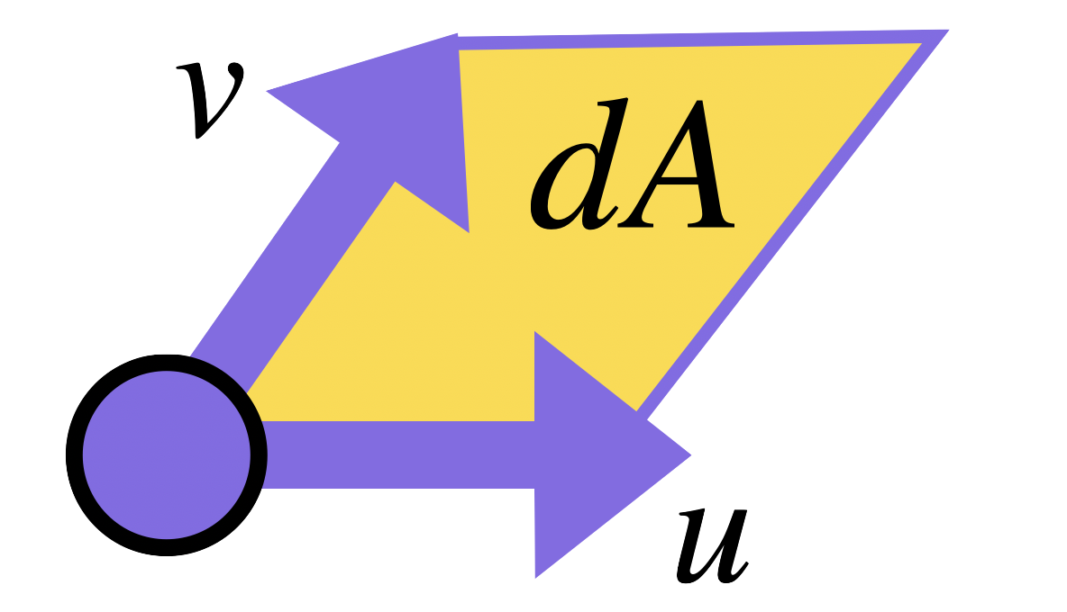
Definition 15.2 (Measuring Infinitesimal area: $dA$) The function $dA$ is an infinitesimal area measure on $T_p{\mathbb{E}}^2$, which takes in two vectors $u,v$ and returns the area of the parallelogram spanned by them:

Area in the tangent space.

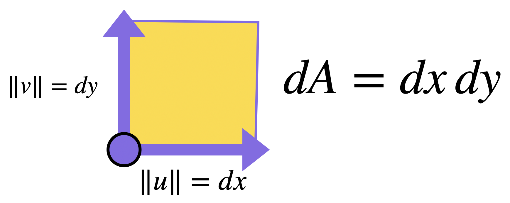
The most common (and useful!) parallelograms that we will encounter are rectangles, due to our use of $x,y$ coordinates on the plane. Here infinitesimal area is quite simple: if the length is $dx$ and the height is $dy$, we have an infinitesimal rectangle with area the product of base and height:

The area of rectangles in the tangent space to a point

Just like lengths, once we have a means of measuring the infinitesimal notion, we can zoom back out to recover what we are really after via integration.

Definition 15.3 (Area in ${\mathbb{E}}^2$) If $R$ is a region in ${\mathbb{E}}^2$, its area is given by the following integral expression $$\mathrm{Area}(R)={\iint }_{R}dA={\iint }_{R}dxdy$$

15.1 Iterated Integrals

How do we compute an integral over a 2-dimensional region, with respect to the infinitesimal area $dxdy$? Looking at a finite approximation gives one answer - we could sum along rows first, adding up all the little areas with the same $y$ coordinates at once. Then we could add up all the total area of each row. In the limit, this tells us to integrate $x$ first, and then *to integrate the result with respect to $y$.

$${\iint }_{R}dA={\iint }_{R}dxdy={\int }_{\mathrm{y}-\mathrm{slices}}\left({\int }_{x-slices}dx\right)dy$$

Conversely, we could have instead sliced our approximation into columns (integrating $dy$ first), and then added up the area of the columns (integrating the results $dx$). This would give

$${\iint }_{R}dA={\iint }_{R}dydx={\int }_{\mathrm{x}-\mathrm{slices}}\left({\int }_{y-slices}dy\right)dx$$

Thus, thanks to the fact that $dA$ factors as a product, an area integral really is just two one dimensional integrals performed in succession! And to evaluate explicit areas, all one needs to do is find a way to measure the length of the $x$-slices or $y$-slices of a region.

In practice, this will be our main means of calculating area. It becomes especially tractable when the region $R$ can be described in terms of single-variable functions, where everything reduces to a 1-dimensional integral!

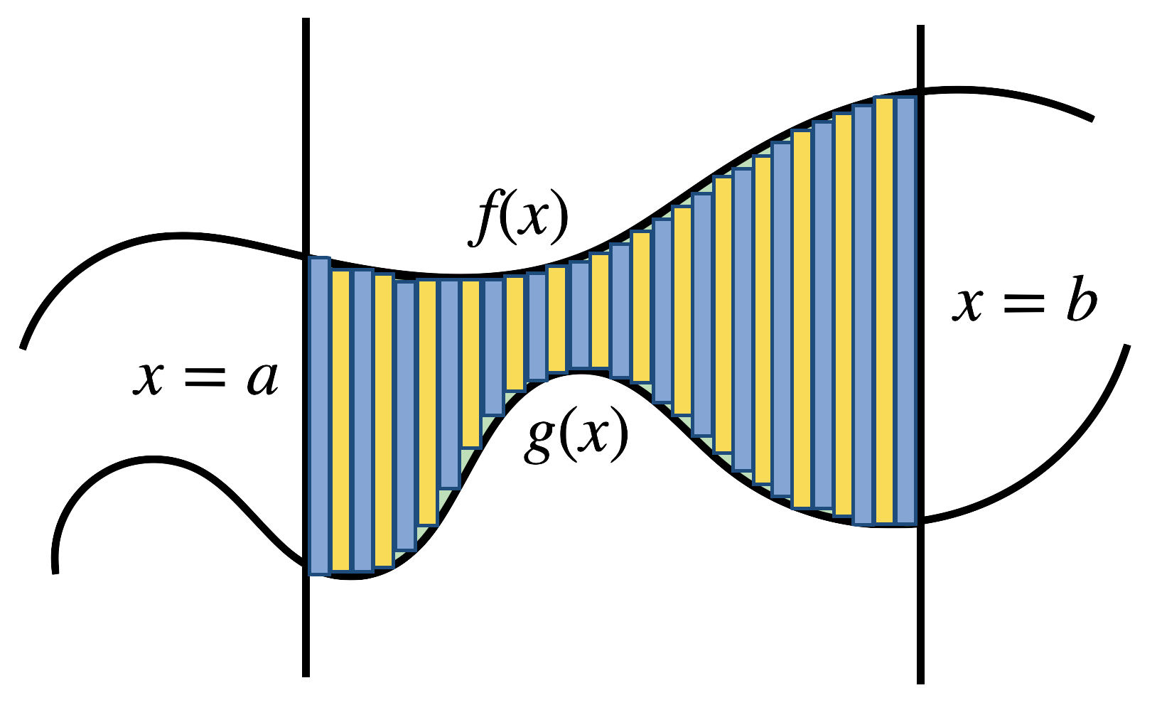
Theorem 15.1 (Area Between Two Curves) Let $f,g$ be functions with $g(x)<f(x)$ on $[a,b]$. Define $R$ as the region $$R=\{(x,y)\mid x\in [a,b],y\in [g(x),f(x)]\}$$

The region between $f(x)$ and $g(x)$.

Then its area can be computed via $$\mathrm{Area}(R)={\int }_a^{b}f(x)-g(x)dx$$

Proof. Then at each fixed $x$, the vertical slice through the region is the interval $[g(x),f(x)]$, and so the area integral can be written as an iterated integral: first over $[g(x),f(x)]$ for a fixed $x$, then over $x\in [a,b]$ $$\mathrm{Area}(R)={\iint }_{R}dA={\int }_{[a,b]}{\int }_{[g(x),f(x)]}dydx$$

The area integral interpreted as an iterated integral, with $\int dy$ done first.

The inner integral here is straightforward to evaluate: there are no $y$’s at all - so by the fundamental theorem we have $${\int }_{[g(x),f(x)]}dy=y{|}_{g(x)}^{f(x)}=f(x)-g(x)$$ Substituting back in gives the result:

$$\mathrm{Area}(R)={\int }_{[a,b]}f(x)-g(x)dx$$

The area between two curves is just the length of all the slices, added up (integrated).

This is how we can define rigorously the area of a circle: we know (for example) that the unit circle has equation $x^2+y^1=1$, and so its top half can be written $y=\sqrt{1-x^2}$ and the bottom half by $y=-\sqrt{1-x^2}$. Thus the area is

$${\int }_{-1}^1{\int }_{-\sqrt{1-x^2}}^{\sqrt{1-x^2}}dydx={\int }_{-1}^{1}2\sqrt{1-x^2}dx$$

Riemann sums for the integral defining the area of a circle with 4,8,16,32, and 64 bars, respectively.

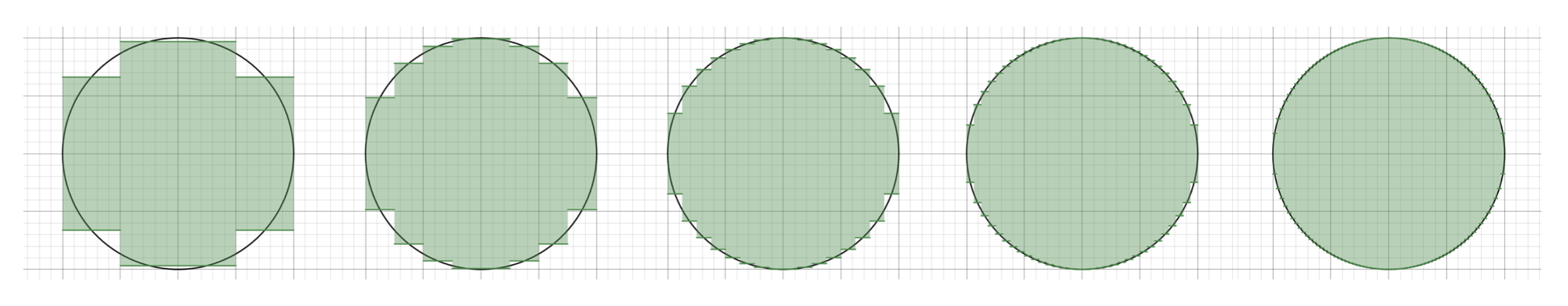
Corollary 15.1 (Defining $\pi$) $$\pi ={\int }_{-1}^{1}2\sqrt{1-x^2}dx$$

Anytime we can describe a region with functions, we are back to calculus. Sometimes this is impossible for an entire region all at once, but we can break it into smaller regions, each of which are described by functions.

Example 15.1 (Area Between Piecewise Curves) Compute the area between the curve $y=\frac{1}{2}{x}^2$ and the piecewise curve below, for $x\in [0,2]$. $$f(x)=\{\begin{array}{ll}{x}^2& x<1\\ x& x\ge 1\end{array}$$

Drawing the region, we decide to divide it into two regions $R_1$ and $R_2$, with $R_1$ the portion with $x\in [0,1]$ and $R_2$ the portion with $x\in [1,2]$.

The region $R$, and its division into two simpler regions $R_1$ and $R_2$.

In each of these regions we can specify the boundaries as functions of $x$, allowing us to express them via single variable integrals (Theorem 15.1) $$\mathrm{Area}(R_1)={\int }_0^1{x}^2-\frac{1}{2}{x}^{2}dx={\int }_0^1\frac{1}{2}{x}^{2}dx=\frac{1}{2}\frac{1}{3}=\frac{1}{6}$$

$$\mathrm{Area}(R_2)={\int }_1^{2}x-\frac{1}{2}{x}^{2}dx=\frac{1}{2}-\frac{1}{6}=\frac{1}{3}$$

The total area is the sum of these, $$\mathrm{Area}(R)=\frac{1}{6}+\frac{1}{3}=\frac{1}{2}$$

We can use this definition of area to compute the area of a triangle in the plane, since we now know how to describe straight lines as affine curves.

Exercise 15.1 (Area of Right Triangle With Calculus) Use calculus to find the area between the $x$-axis, the $y$-axis, and the linear equation with $y$-intercept $(0,h)$ and $x$-intercept $(b,0)$.

Exercise 15.2 (Area of a General triangle) Set up an area integral to measure the area of a triangle with vertices $O$, $(L,0)$, and $(p,q)$ (assume $L,p$ and $q$ are positive numbers: it will be a piecewise area between curves).

Triangles for various $p,q,L$.

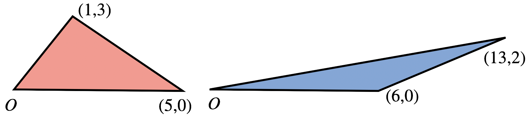
Show the result gives you half the base times the height.

Similarly, we can make quick work of some impressive results of archimedes, after checking that $y=x^2$ actually describes a parabola (in Exercise 13.8)

Exercise 15.3 (Quadrature of the Parabola with Calculus)  

• Write down a formula for the area of the triangle whose third vertex lies at $(x,x^2)$
• Use calculus to find the point $x$ where the inscribed triangle has maximal area. Then show that Archimedes was right: the slope of the tangent line to the parabola at this point is exactly the same as the slope of the line segment forming the triangle’s base!
• Finally, compute the area of the parabolic segment (via integration, as the area between two curves). Show that its exactly $4/3$rds the area of the triangle!

(Hint: instead of finding the height of the triangle to use $\frac{1}{2}bh$, can you use the fact that the determinant of a matrix calculates the area of a parallelogram whose sides are the column vectors, and that the area of a the triangle you want is half a parallelogram?)

15.2 Isometries & Similarities

Now that we know how to evaluate an area integral, its time to study some of its properties. Our first question with every new concept we define should be how does this concept interact with isometries? So we investigate this below.

Theorem 15.2 (Isometries Preserve Area) Let $R$ be a region in the plane, and $\varphi$ an isometry. Then $$\mathrm{Area}(\varphi (R))=\mathrm{Area}(R)$$

Proof. Let $R$ be a region in the plane, and at each point $p\in R$ consider the unit orthogonal vectors $e_1=⟨1,0{⟩}_p$ and $e_2=⟨0,1{⟩}_p$ defining the unit area square used in the computation of $dA$. Since isometries preserve infinitesimal lengths and angles, $\varphi$ takes this to another infinitesimal unit square based at $\varphi (p)$, also of unit area.

Angles and infinitesimal lengths are preserved, so infinitesimal squares are sent to squares of the same area.

Thus, the integral ${\iint }_{\varphi (R)}dA$ is adding up the exact same areas as ${\iint }_{R}dA$, and they are equal.

Theorem 15.3 (Similarities Scale Area) Let $R$ be a region in the plane, and $\sigma$ an similarity with scaling factor $k$. Then $$\mathrm{Area}(\sigma (R))=k^2\mathrm{Area}(R)$$

Proof. Running a similar argument to the above, we see that the infinitesimal unit square defined by $e_1=⟨1,0{⟩}_p$ and $e_2=⟨0,1{⟩}_p$ at each point is taken to a square with side lengths $k$ (since similarities uniformly scale infinitesimal lengths, but still preserve angles).

Angles are preserved but infinitesimal lengths are scaled by $k$. Thus infinitesimal areas are scaled by $k^2$.

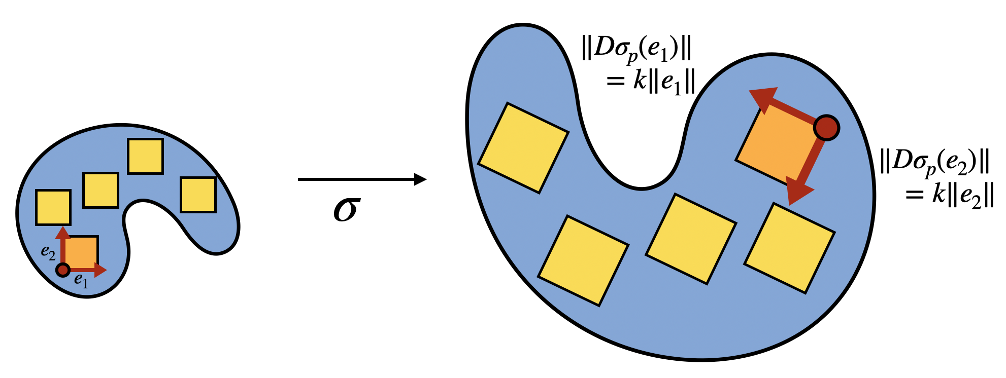
The area of such a square is $k^2$, so the integral defining $\mathrm{Area}(\varphi (R))$ counts an area of $k^2$ every time the integral defining $\mathrm{Area}(R)$ counts a unit area. Thus, the total area is $k^2$ times the original.

15.3 Area and General Mappings

Both isometries and similarities are rather special: they send every infinitesimal unit square to another square, possibly scaled in size by a constant factor.

In this section we are interested in discovering what happens to an area under a general map ${\mathbb{E}}^2\to {\mathbb{E}}^2$. First, let’s consider a conformal map $\varphi$. This map takes infinitesimal squares to squares, but they no longer all need to be the same size.

Conformal maps take infinitesimal squares to squares, but the size of the square can differ across the region.

Indeed, by Corollary 14.8 we know that at each point $p\in {\mathbb{E}}^2$ the sides of such an infinitesimal square are $⟨a,b⟩$ and $⟨-b,a⟩$ - each of length $\sqrt{a^2+b^2}$ so the total infinitesimal area is scaled up from $1$ by $a(x,y{)}^2+b(x,y{)}^2$. (Here we’ve written $a$ and $b$ as functions of $x,y$ to emphasize that they may take different values at different points of the plane).

Thus the area of the region $\varphi (R)$ can be computed starting from $R$, but multiplying each infinitesimal area by this factor:

$$\mathrm{Area}(\varphi (R))={\int }_R(a(x,y{)}^2+b(x,y{)}^2)dxdy$$

Example 15.2 (Area under the map $z\mapsto z^2$) The squaring map from complex analysis can be written as a function of real coordinates $x,y,$ as $$S(x,y)=(x^2-y^2,2xy)$$ This map takes the unit square $R=\{(x,y)\mid x\in [0,1],y\in [0,1]\}$ to the region $S(R)$ depicted below.

The image of the unit square under the complex squaring map.

Using all that we’ve learned, we can actually compute the area of this region without having to even describe it explicitly! We know that at each point $(x,y)$, the derivative map is

$$D{F}_p=\left(\begin{array}{cc}2x& -2y\\ 2y& 2x\end{array}\right)$$

Thus the change in area for the infinitesimal square based at $(x,y)$ is $4(x^2+y^2)$. This allows us to compute the area as $$\mathrm{Area}(S(R))={\iint }_{R}4(x^2+y^2)dxdy$$ Which we can now just do as an iterated integral:

$$\begin{array}{rl}{\iint }_{R}4(x^2+y^2)dxdy& ={\int }_0^1({\int }_0^{1}4(x^2+y^2)dx)dy\\ & ={\int }_0^{1}4(\frac{x^3}{3}+x{y}^2){|}_0^{1}dy\\ & ={\int }_0^1\frac{4}{3}+4y^{2}dy\\ & =(\frac{4}{3}y+\frac{4}{3}{y}^3){|}_0^1\\ & =\frac{8}{3}\end{array}$$

Finally, let’s consider a general map $F:{\mathbb{E}}^2\to {\mathbb{E}}^2$ of the plane. We know $F$ does not need to preserve infinitesimal lengths or angle, and so takes takes squares in the tangent space to rectangles or parallelograms.

A general mapping need not preserve angles or lengths, and so will take the original infinitesimal squares defining $dA=dxdy$ to parallelograms of various sizes and shapes.

But we can figure out from this what $F$ does to infinitesimal areas: it takes the unit area spanned by $⟨1,0⟩$ and $⟨0,1⟩$ to the parallelogram spanned by $D{F}_p(⟨1,0⟩)$ and $D{F}_p(⟨0,1⟩)$!

The area of the parallelogram determined by these two vectors is just the determinant of $DF$!

And we know how to calculate the area of a parallelogram using the vectors determining its sides (Exercise 14) - this is just the determinant of the derivative matrix.

Theorem 15.4 If $F:{\mathbb{E}}^2\to {\mathbb{E}}^2$ is any differentiable mapping, $F$ takes the unit infinitesimal area in $T_p{\mathbb{E}}^2$ to the area $$|detD{F}_p|=\left|\begin{array}{cc}{\partial }_x{F}_1& {\partial }_y{F}_1\\ {\partial }_x{F}_2& {\partial }_y{F}_2\end{array}\right|={\partial }_x{F}_1{\partial }_y{F}_2-{\partial }_y{F}_1{\partial }_x{F}_2$$ This quantity is called the Jacobian of $F$ at $p$.

Much like we have done for isometries, similarities, and conformal maps before; this lets us compute the area of a region $F(R)$ as an integral directly over the starting region $R$ itself! At each point $p\in R$ we just insert the area scaling factor for how much $F$ changes the area of an infinitesimal square based there: the Jacobian.

Theorem 15.5 Let $R\subset {\mathbb{E}}^2$ be a region in the plane, and $F:{\mathbb{E}}^2\to {\mathbb{E}}^2$ some mapping that takes $R$ to a new region, $F(R)$. Then

$$\mathrm{Area}(F(R))={\int }_{F(R)}dA={\int }_R|detDF|dxdy$$

We can use this to find areas that seem difficult at first: for example, we will be able to calculate the area of an ellipse in terms of the area of a circle (we’ll find the circles’ area in the next section).

Exercise 15.4 The map $F(x,y)=(ax,by)$ takes points on the unit circle to the points of the ellipse $\frac{x^2}{a^2}+\frac{y^2}{b^2}=1$. (Confirm this with algebra!) Thus, it takes the unit disk $D=\{(x,y)\mid x^2+y^2\le 1\}$ to the interior of this ellipse: call this region $E$.

Stretching a circle into an ellipse.

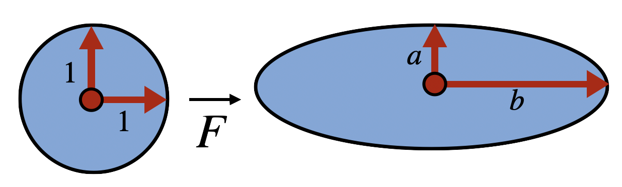
Computing the Jacobian we see $F$ scales areas by a factor of $ab$: $$DF=\left(\begin{array}{cc}a& 0\\ 0& b\end{array}\right)⟹|DF|=det\left(\begin{array}{cc}a& 0\\ 0& b\end{array}\right)=ab$$

This stretches all infinitesimal areas by a factor of $|DF|=ab$

Thus we can calculate the area of the ellipse $E$ as

$$\begin{array}{rl}\mathrm{Area}(E)& ={\iint }_{E}dA\\ & ={\iint }_{F(D)}dA\\ & ={\iint }_D|DF|dxdy\\ & =\iint abdxdy\\ & =ab{\iint }_{D}dxdy\\ & =ab\mathrm{Area}(D)\end{array}$$

We will see in shortly that $\mathrm{Area}(D)=\pi$, so that immediately gives $\mathrm{Area}(E)=\pi ab$.

One thing to be careful about: while all isometries preserve area, not all area-preserving maps are isometries! Take any determinant 1 matrix on the plane and use it as a linear map. This preserves area of all subsets (as derivative is itself, and so determinant of the derivative is 1). But does not preserve lengths: try a hyperbolic like $$\left(\begin{array}{cc}2& 0\\ 0& 1/2\end{array}\right)$$

15.4 The Jacobian, Abstractly

This optional section gives a second means of deriving the jacobian, instead of taking the fact that we already understand the area of a parallelogram. We could instead ask, what sort of behavior do we want the function $dA$ to have; and try to derive its formula from such a list.

Instead of being explicit about what number $dA$ assigns to every area, we can attempt to be more austere and just declare that $dA$ assigns the unit square $⟨1,0⟩,⟨0,1⟩$ unit area.

To get further than this, we need a proposal about how $dA$ interacts with scalar multiplication. If $v,w$ are two vectors and we multiply one of them by $k$, this should increase the area they span by $k$: that is, $$dA(kv,w)=kdA(v,w)$$

For vector addition, we analogously propose that the area spanned by $u+v$ and $w$ is the same as the area spanned by $u,w$ and $v,w$

$$dA(u+v,w)=dA(u,w)+dA(v,w)$$

We’ve illustrated the case of addition and scalar multiplication in the first vector above, but of course it should not depend which vector we are talking about, so we propose that $dA$ is linear in each of its input vectors.

We have one final thing to consider: what is the relationship between $dA(v,w)$ and $dA(w,v)$? A natural thought is that these both describe the same area, an so should certainly be assigned the same number! But this is ignoring a useful piece of information: that switching between $(v,w)$ and $(w,v)$ negates the sense of angles, essentially flipping the parallelogram. To allow $dA$ to record this information, we may impose that switching the input vectors negates the result. (Multi)-linear functions with this property are called alternating $$dA(v,w)=-dA(w,v)$$

In fact, these properties alone are enough to fully determine the function $dA$! And, evaluating it on an arbitrary pair of input vectors, we see the usual formula for the determinant is forced on us.

Exercise 15.5 Using only the following facts about the function $dA(v,w)$, derive the standard formula for the determinant $$dA(\left(\begin{array}{c}a\\ c\end{array}\right),\left(\begin{array}{c}b\\ d\end{array}\right))=ad-bc$$

• $dA$ evaluates to 1 on the square $⟨1,0⟩,⟨0,1⟩$.
• $dA$ is alternating: $dA(v,w)=-dA(w,v)$.
• $dA$ is linear in both the first and second argument.