30 Geometry of Minkowski Space
Our introduction to Minkowski space in the last chapter essentially provided a playground for us geometers,
- We got to try out our definitions (of isometries, distances, etc) in an unfamiliar context, which was still quite close to things we’ve seen before (all we switched was one negative sign in the dot product!)
- We were able to use our geometric skills to discover a new model of hyperbolic geometry living inside this world!
This provides a nice end to our story of hyperbolic space, and our approach to geometry as a whole. But it also serves as the beginning to a new and wonderful story of geometry and its interaction with physics. In these final chapters we endeavour to tell a small bit of this story, where Minkowski space itself (and not merely the hyperboloid lying within it) takes center stage.
To begin, we need to take a deeper dive into the geometric properties of Minkowski space.
30.1 Positive and Negative
As a geometry, Minkowski space is a \(n+1\) dimensional real vector space \(M\) where each tangent space space \(T_pM\cong\RR^{n,1}\) comes equipped with the inner product \(\star\).
At each point \(p\in M\) there is a null cone of vectors of length zero. Any isometry of \(M\) preserves null cones: it sends the null cone at \(p\) to the null cone at \(\phi(p)\).
One of the most effective ways to study a geometric space is with curves: for example, in Riemannian geometry we used curves to help us define geodesics, and then learned a ton of geometry from trying to classify geodesics. Let’s attempt the same here.
First, we recall the definition of a regular curve. In Riemannian geometry, we said this is a curve \(\gamma\colon I\to M\) where the derivative is never zero (or, equivalently, its norm is never zero). We copy this definition in Minkowski space
Definition 30.1 (Regular Curve:) A curve \(\gamma \colon I\to M\) is regular if \(\|\gamma^\prime(t)\|\neq 0\) for all \(t\in I\).
However note here that \(\gamma^\prime\neq 0\) is not equivalent to \(\|\gamma^\prime\|\neq 0\) as there are null vectors. Nonetheless the definition we chose for regular is the “correct” one, as the reason one imposes regularity on curves is that one often wishes to do computations that require dividing by \(\|\gamma^\prime|\).
This condition makes the collection of regular curves in Minkowski space quite different than in Riemannian geometry: we can sort all regular curves into two classes (which for now, we will call positive and negative).
Definition 30.2 (Positive and Negative Curves.) We say a regular curve is positive if \(\gamma^\prime(t)\) has positive norm for all \(t\), and is negative if the norm is negative for all \(t\).
Theorem 30.1 Regular Curves are Either Positive or Negative. Precisely, let \(\gamma\) be a regular curve: then it is either a positive or negative curve.
Proof. Apply the intermediate value theorem to the function \(\|\gamma^\prime\|\).
Of the non-regular curves, most have points of positive and negative norm - but a few special ones do not: they have zero norm everywhere. These are worthy of a special name
Definition 30.3 A curve \(\gamma\) is null if \(\|\gamma^\prime(t)\|=0\) for all \(t\).
This sorting of all regular curves curves into two classes has profound implications: it let’s us actually sort the points of \(M\) into classes
Definition 30.4 (Positive and Negative Pairs of Points.) Let \(p,q\in M\) be two points. We say that \(p\) and \(q\) are positively separated if there is a positive curve starting at \(p\) and ending at \(q\). They are negatively separated if there is a negative curve starting at \(p\) and ending at \(q\). And, they are null separated if there is a null curve connecting them.
This definition requires some checking to be sure its well-defined:
Theorem 30.2 If two points are connected by a negative curve, then any regular curve connecting them must be negative. Same for positive pairs. Hint: A sneaky use of Rolle’s theorem to the z coordinate, for negative curves!
Using affine lines (which are easy to tell when they are positive or negative curves, just using the norm of their derivative) we can sort points into positives and negatives with this definition.
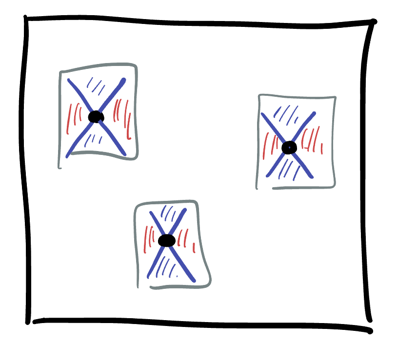
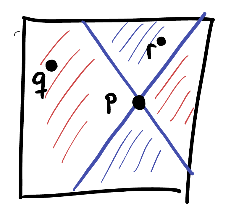
Exercise 30.1 For the origin, show that the points that are positively separated from \(O\) are those outside (horizontally) of the X made by the lines \(z=\pm x\), and the points that are negatively separated are inside (vertically above an d below) the X.
This same thing holds true at every point: given a point \(p\in M\) we can sort all other points \(q\) so that the positive pairs (p,q) are all the points lying outside of an X centered at \(p\) and the negative paris are all the points inside that same \(X\).
30.1.1 Geodesics
Now that we understand a bit of isometries, regular curves, and positively/negatively separated points, we can start to talk about geodesics in Minkowski space. This discussion is more subtle than in Riemannian geometry, for several reasons.
We’ve already dealt with one major difference: the fact that not all pairs of points in Minkowski space are created equal - for some pairs, every regular curve connecting them is a positive curve, and for others every regular curve is a negative curve (and finally, for the remaining pairs of null-separated points, there are no regular curves at all joining them).
Thus, we already expect there to be two notions of geodesic, a positive geodesic as some optimization problem over the space of positive curves, and correspondingly a negative geodesic for pairs of negatively separated points.
But there’s one more subtlety to confront: we already know that Minkowski space has curves of total length zero between distinct points. This radically different behavior that Euclidean space suggests a potential problem with our usual notion of geodesic as minimizing - if we can make a regular curve nearby to a curve of zero length, we might expect that regular curve to have a very short length - and perhaps taking the infimum over all regular curve lengths actually gives zero, which is not realized by any regular curve.In fact, exactly this worry happens.
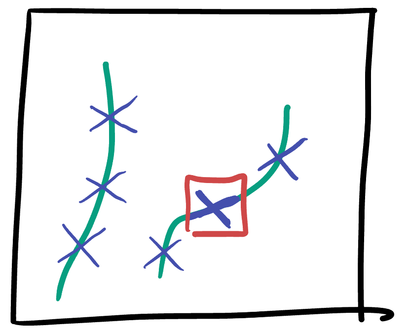
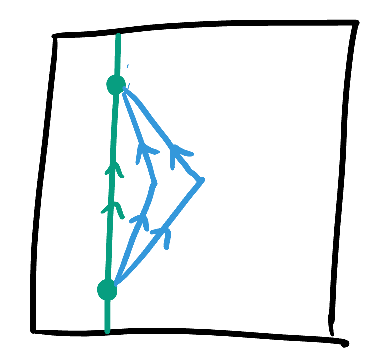
Theorem 30.3 (A truly mindbending example) Consider the following two curves in \(\RR^{2,1}\): the first curve \(\gamma\) is just the vertical segment from \((0,0)\) to \((0,4)\). THe second curve \(c\) is piecewise: it begins with the affine line segment connecting \((0,0)\) to \((1,2)\) and then continues as the affine line segment connecting \((1,2)\) to \((0,4)\).
Which is longer? Now do the same for the piecewise curve that bends at the point \((a,2)\) instead of \((1,2)\), for \(a\in [0,2]\). Show that there is a curve connecting \((0,0)\) to \((0,4)\) with arbitrarily short nonzero length:
Exercise 30.2 Can you construct a similar example, for a pair of positively separated points?
One concern here might be that these curves described are not regular - they have a corner (they are piecewise regular, however). This is not actually a technical concern as it is fine (and often more convenient) to just work with the class of piecewise regular curves from the start. But even if you choose not to do so, these examples still point the way:
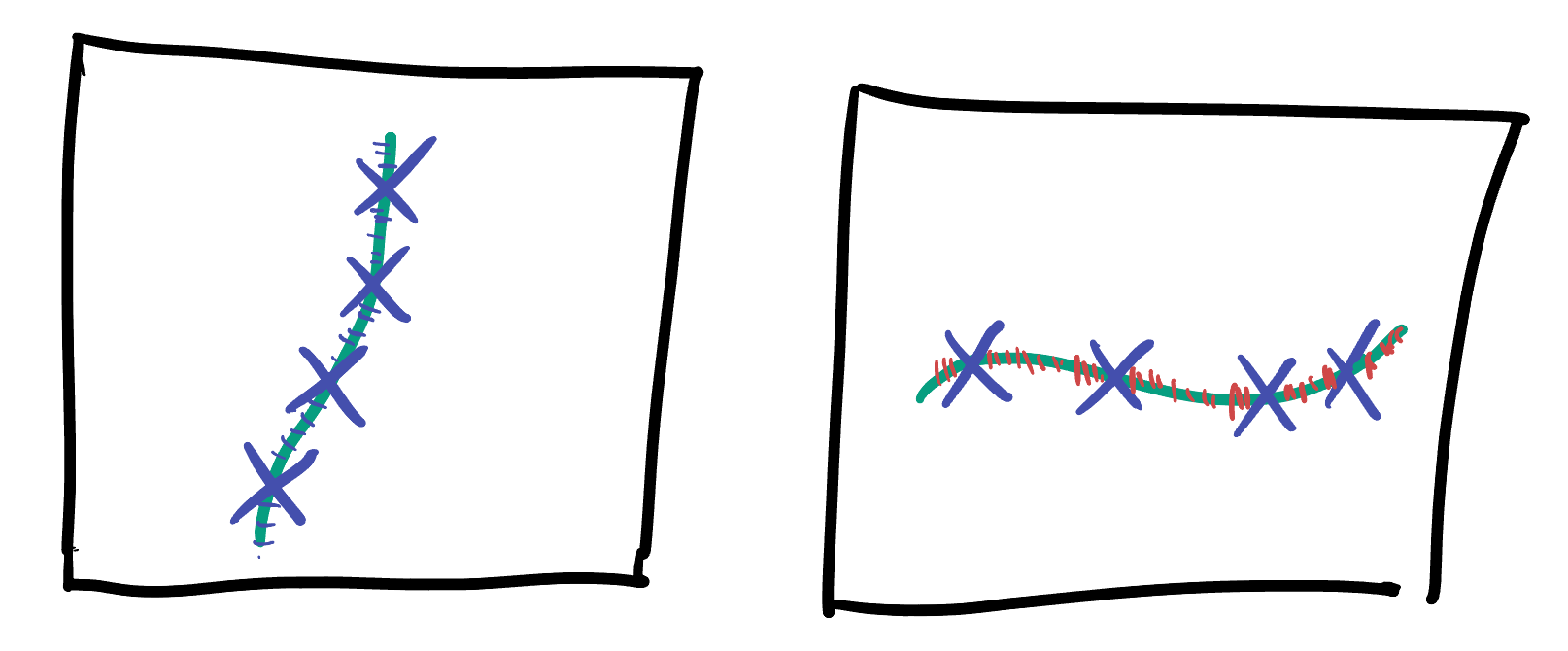
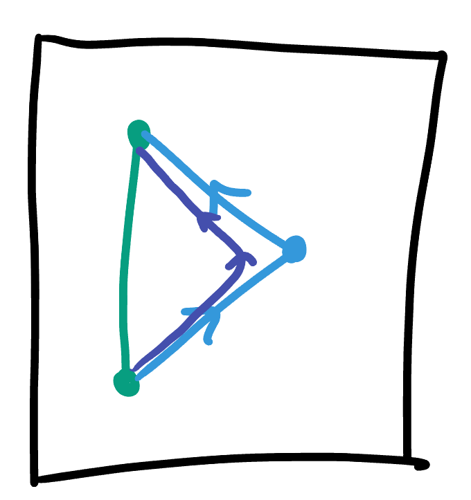
Example 30.1 Given two negatively separated points (without loss of generality we can take them to be \((0,0)\) and \((0,a)\) after applying isometries), there are regular curves of arbitrarily short length connecting them. The idea is to approximate the piecewise curve above by something smooth, in this case, a segment of a hyperbola
The situation is even worse that these examples make it appear - here we found curves that were very short, but were also very far away from our original curve. Perhaps one might hope there aren’t any actually nearby to our original curve - so maybe its still “locally” nice. But this intuition is rather shaky; by modifying the idea above to introduce lots of small crinkles instead of one big deviation….
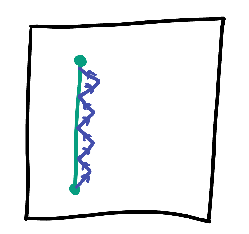
Exercise 30.3 If you constrain a curve to never get more than \(\epsilon\) away from a vertical line in its \(x\) coordinate, what can you say about its length? Can it be arbitrarily close to zero, or is there some lower bound?
What about if its a regular curve?
Corollary 30.1 There are no length minimizing regular curves in Minkowski space: given any pair of positively or negatively separated points, the infimum of the lengths of all regular curves joining them is zero, but there is no regular curve of length zero joining them.
Thus, the inifmum is not a minimum, so the minimum does not exist!
This example teaches us two important things: first the formal definition of geodesic can’t be directly borrowed from Riemannian geometry, but secondly we can see its clearly not even the right notion! In Riemannian geometry, its easy to make a curve longer, by wiggling it, curves of minimal length are the right sort of optimal objects to seek. But in Minkowski space, its easy to make a curve shorter by wiggling it; and in fact, its difficult to make a curve longer! Almost everything you try shortens it…so perhaps the right thing to do is turn our intuition on its head and define our optimal objects as the length maximizing curves. Amazingly, for negative curves this works!
Definition 30.5 (Negative Geodesics) Let \(p,q\) be two negatively separated points in Minkowski space. Then in the set of all regular curves joining \(p\) to \(q\), there is a unique curve of maximal length.
We call this curve the geodesic from \(p\) to \(q\).
This is a definition that justifies itself with a claim: (that there is a maximum, and as a bonus its unique!) So, we should check this!
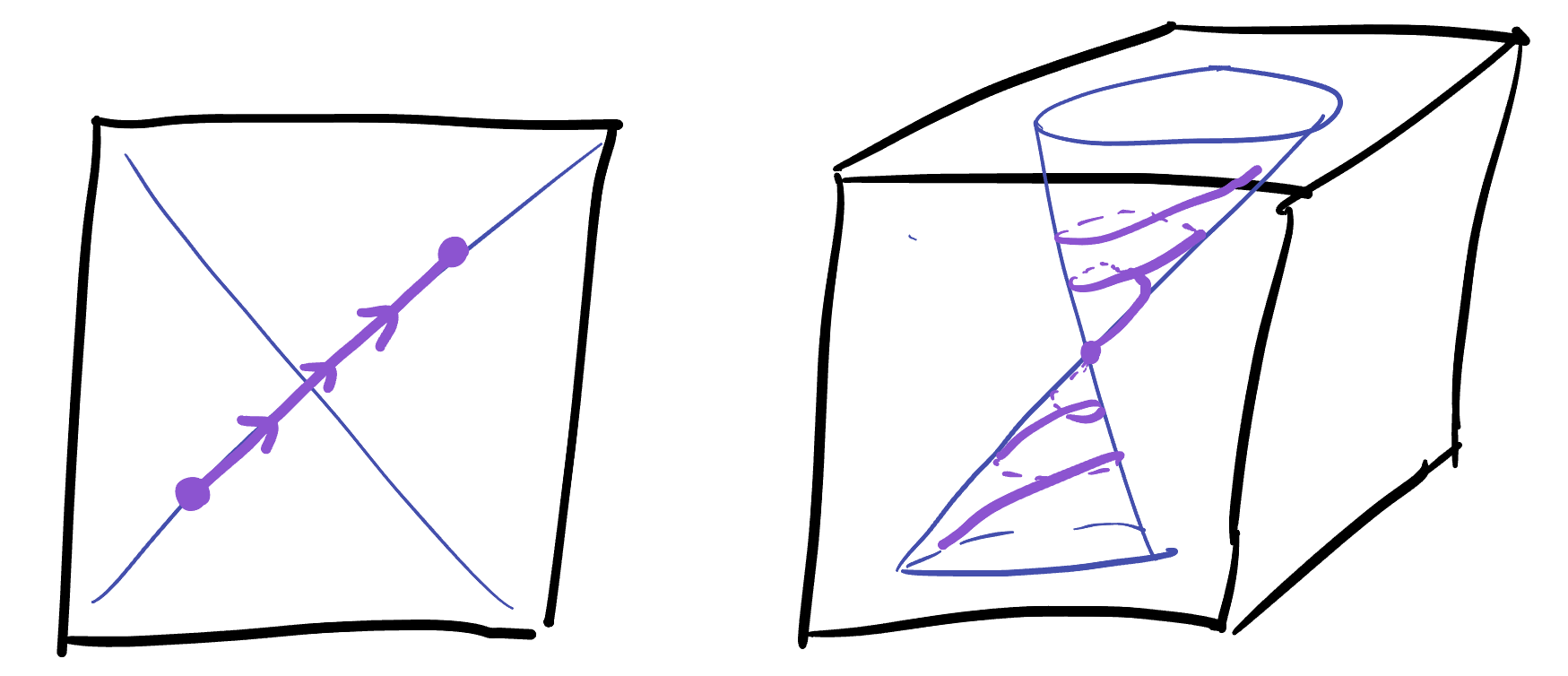
Theorem 30.4 If \(\gamma\) is an affine line connecting two negatively separated points, then \(\gamma\) is globally length maximizing.
Proof. Without loss of generality we can take our points to be \((0,0)\) and \((0,a)\) after using some isometries, and so \(\gamma\) is the curve \(\gamma(t)=(0,t)\). Now let \(\alpha(t)=(x(t),z(t))\) be any other curve joining \(\alpha(0)=(0,0)\) and \(\alpha(1)=(0,a)\). Writing out its length, we see
\[\begin{align*} \operatorname{Length}(\alpha)&=\int_I \sqrt{|\alpha^\prime\star\alpha^\prime|}\,dt\\ &=\int_I \sqrt{|(x^\prime)^2-(z^\prime)^2|}\,dt\\ &=\int_I \sqrt{(z^\prime)^2-(x^\prime)^2}\,dt \end{align*}\]
Where the last equality follows as since \(\alpha\) is regular and joins negatively separated points, we know that \(\alpha^\prime(t)\) is negative for all \(t\), and so taking the absolute value is the same as multiplying by a negative.
But, no matter what \(x(t)\) is we know \(x^\prime(t)^2\geq 0\) and so for all \(t\)< \[(z^\prime)^2-(x^\prime)^2\leq (z^\prime)^2\]
Both sides of this are positive and the square root is an increasing function, so this implies
\[\sqrt{(z^\prime)^2-(x^\prime)^2}\leq \sqrt{(z^\prime)^2}=|z^\prime|\]
and finally, \(|z^\prime|\geq z^\prime\), so stringing these inequalities together and integrating yields
\[\int_I \sqrt{(z^\prime)^2-(x^\prime)^2}\,dt \leq \int_I z^\prime\, dt\]
The first integral here is none other than the length of \(\alpha\), and the second integral here is easily evaluated via the fundamental theorem of calculus:
\[\int_{[0,1]}z^\prime\,dt = z(1)=z(0)=a-0=a\]
Thus for any such curve \(\alpha\) we have \(\operatorname{Length}(\alpha)\leq a\). As this is precisely the length of the affine line \(\gamma\) we have
\[\operatorname{Length}(\alpha)\leq \operatorname{Length}(\gamma)\]
As a corollary of this, looking closer at the argument above we can see that in fact no other curve can be as long as \(\gamma\), so this is the unique maximum
Exercise 30.4 Geodesics connecting negatively separated points are unique.
Hint: if \(\alpha\) is distinct from \(\gamma\) then its \(x\) coordinate must be nonzero at some point. Because it is continuous, this means there must be some small interval where the \(x\) coordinate is nonzero, and on this interval you can show the length of \(\alpha\) is strictly less* than the length of \(\gamma\). On the rest of the curve we can get \(\leq\) as above, and putting it together we get the inequality is strict: \(\alpha\) must actually be shorter than \(\gamma\)!
In fact, there’s a way to make this craziness sound not so strange after all. Remember that we defined infinitesimal arclength by using an absolute value for negative curves, since the dot product yields a negative number. So, finding the maximal length is really finding the maximum absolute value which is the same as finding the most negative (since we know the original numbers are all negative). But the most negative is the minimum! So, we could simply modify our definition of the length of a negative curve to remember that the dot product is negative
\[L(\gamma)=-\int_I \sqrt{|\gamma^\prime\star\gamma^\prime|}\,dt\]
And with this new definition all curves have negative length, the maximum is not achieved (as curves can have lengths arbitrarily close to zero) but the minimum is: curves of minimal length are again geodesics! This is a totally fine approach to take, and perhaps a convenient one if you are very good at not missing minus signs. However when it comes to our use case for Minkowski geometry (the physics of relativity) we will see that the length of negative curves really corresponds to time intervals, and if we put a negative here, we’ll have to negate it once more to think of intervals of time as positive like we do in daily life. So, we will opt not to do this, and instead just deal with the fact that geodesics are maximizing.
This turns out to be alright actually - as its strangeness actually forces us to think carefully about what is going on, and this careful though reveals things are even stranger for positively separated points!
In \(\RR^{1,1}\) where the inner product has one positive and one negative direction, things are symmetric, and so nothing stranger happens (positive geodesics are also length maximizing). But, as soon as there is more than one positive direction, things can get rather strange indeed.
Exercise 30.5 Let \(p=(0,0,0)\) and \(q=(2,0,0)\) be two positively separated points in \(\RR^{2,1}\), and let \(\gamma(t)=(t,0,0)\) be the affine line connecting them.
- Show that there are nearby curves to \(\gamma\) which are shorter, by varying the curve slightly into the negative \(z\) direction (for example, look at the curve connecting \((0,0,0)\) to \((1,0,z)\) and then continuing to \((2,0,0)\) for \(z\in(0,1)\).)
- Show that there are nearby curves to \(\gamma\) which are longer
To study this a bit further, it will be useful to have a little more terminology available to us, so we introduce the idea of a variation:
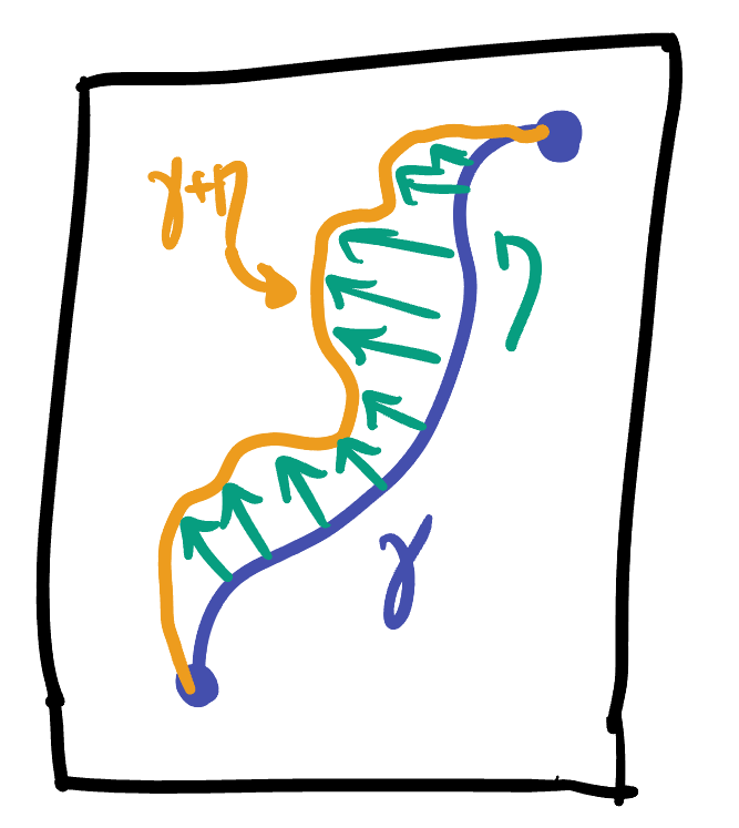
Definition 30.6 If \(\gamma\) is an affine line between two positively separated points, a variation of \(\gamma\) is a nearby curve \(\gamma+\eta\), where \(\eta\) is some curve with \(\eta(a)=\eta(b)=0\) (so that \(\gamma\) and its variation start and end at the same point).
We call \(\gamma+\eta\) a negative variation if \(\eta(t)=(0,0,z(t))\) is nonconstant only in the direction where the inner product returns negative values, and analogously we call \(\gamma+\eta\) a positive variation if \(\eta(t)=(x(t),y(t),0)\) is non-constant only in the directions where \(\star\) is positive.
Exercise 30.6 Let \(p,q\) be two positively separated points in Minkowski space, and \(\gamma\) the affine line connecting them.
- Show that \(\gamma\) is a local minimum of the length functional over the set of all positive variations of \(\gamma\).
- Show that \(\gamma\) is a local maximum of the length functional over the set of all negative variations of \(\gamma\).
This shows that \(\gamma\) is a local minimum of length if you vary the curve in the positive directions of the inner product, but is a local maximum if you instead vary the curve a bit in the negative direction. From multivariable calculus we might recognize points that are either a maximum or minimum depending on the direction you slice in as saddle points, and indeed this is the case here.
Theorem 30.5 Let \(p,q\) be a pair of positively separated points in Minkowski space, and \(\gamma\) the affine line connecting them. Then \(\gamma\) is a saddle point of the length functional over all regular curves.
We do not prove this theorem, as understanding the precise definition of a saddle point in infinite dimensions, and ensuring to do the calculation correctly would take us rather far afield. And, seeing that we will never use this result (in our upcoming physics application, it will turn out that only the negative curves are relevant) its just not worth it here.
However, it does tell us that if we want a general definition of geodesic in Minkowski space, we need to work a little harder: we can’t just replace local minimum with local maximum and call it a day; instead we should seek a definition which captures both max/mins and saddles.
Definition 30.7 (Minkowski Geodesics) A minkowski geodesic is a regular curve \(\gamma\colon\RR\to\RR^{3,1}\) which is a critical point of the Length functional \[\mathrm{Length}(\gamma)=\int_I\|\gamma^\prime\|\,dt = \int_I \sqrt{|\gamma^\prime\star\gamma^\prime|}\,dt\]
In fact, one could take this more general definition and apply it back in Riemannian geometry as well. Even though it appears to allow for more possible behaviors, one can prove that with a positive inner product at each tangent space, the only critical points of length are actually minima - that is, they are the same geodesics we have already found! So, there is no harm in replacing the definition with this, and using it universally across both Riemannian and Minkowski spaces.
This small change turns out to be the a hint to much wider generalizations, bringing geometry deep into the study of quite a lot of fields of math and physics. We do not have the time nor background to develop such here, and should remain focused on our goal. But I cannot help but mention one: Lagrange managed to rewrite the laws of classical mechanics as an optimization problem, where the solutions to Newton’s laws appeared to correspond to the minima of a certain function (called the Action Functional). But on closer inspection - this didn’t always work! Instead we discovered physics is not seeking minima but rather critical points and so this generalized notion of geodesic is the correct notion here as well. (Look up The Principle of Stationary Action to learn more)