Assignments
Problem Set I
Exercise 1 (Constructing an Isoceles Triangle) Start with a line segment of length \(a\). Prove that you can construct a triangle with one side of length \(a\), and two sides of length \(2a\).
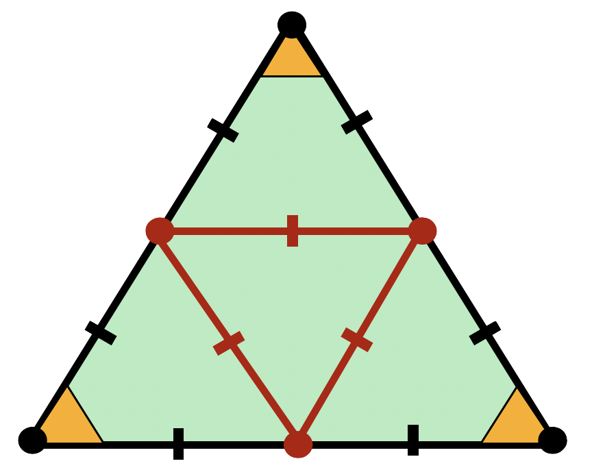
Exercise 2 (Inscribing an Equilateral Triangle) Prove that inside of an equilateral triangle, you can inscribe an upside down equilateral triangle of exactly half the side length, shown
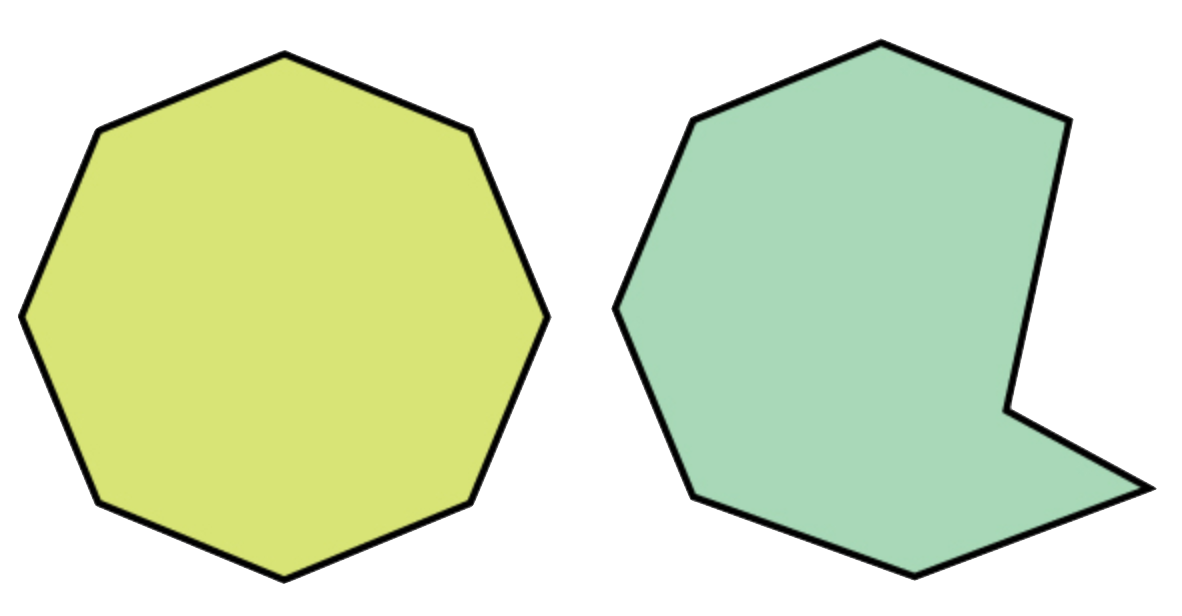
Exercise 3 (Angle Sums of Polygons) A polygon is convex if all of its angles are less than \(180^\circ\), so that it has no “indents”. Equivalently, a convex polygon is one where any line segment with endpoints on the boundary of the polygon lies inside the polygon.
Prove that the angle sum of convex quadrilaterals is a constant, for all quadrilaterals. Prove the angle sum of convex pentagons is also a constant. What are these constants?
What do you think the formula is for the sum of angles in a convex \(n\)-gon? (Optional: If you have seen mathematical induction, prove your guess!)
Exercise 4 (Rectangles Exist) Prove that Rectangles exist using Euclid’s Postulates (and also Playfair’s Axiom, if you like it), and the propositions proven in the sections Euclid and Parallels.
Hint - we know how to make right angles now, and parallel lines through points. Start making some!
Exercise 5 (Diagonal Bisectors) If the diagonals of a quadrilateral are bisect one another, then that quadrilateral is a parallelogram.
Exercise 6 (Proving the Pythagorean Theorem) The following is an ingenious rearrangement proof of the Pythagorean theorem.
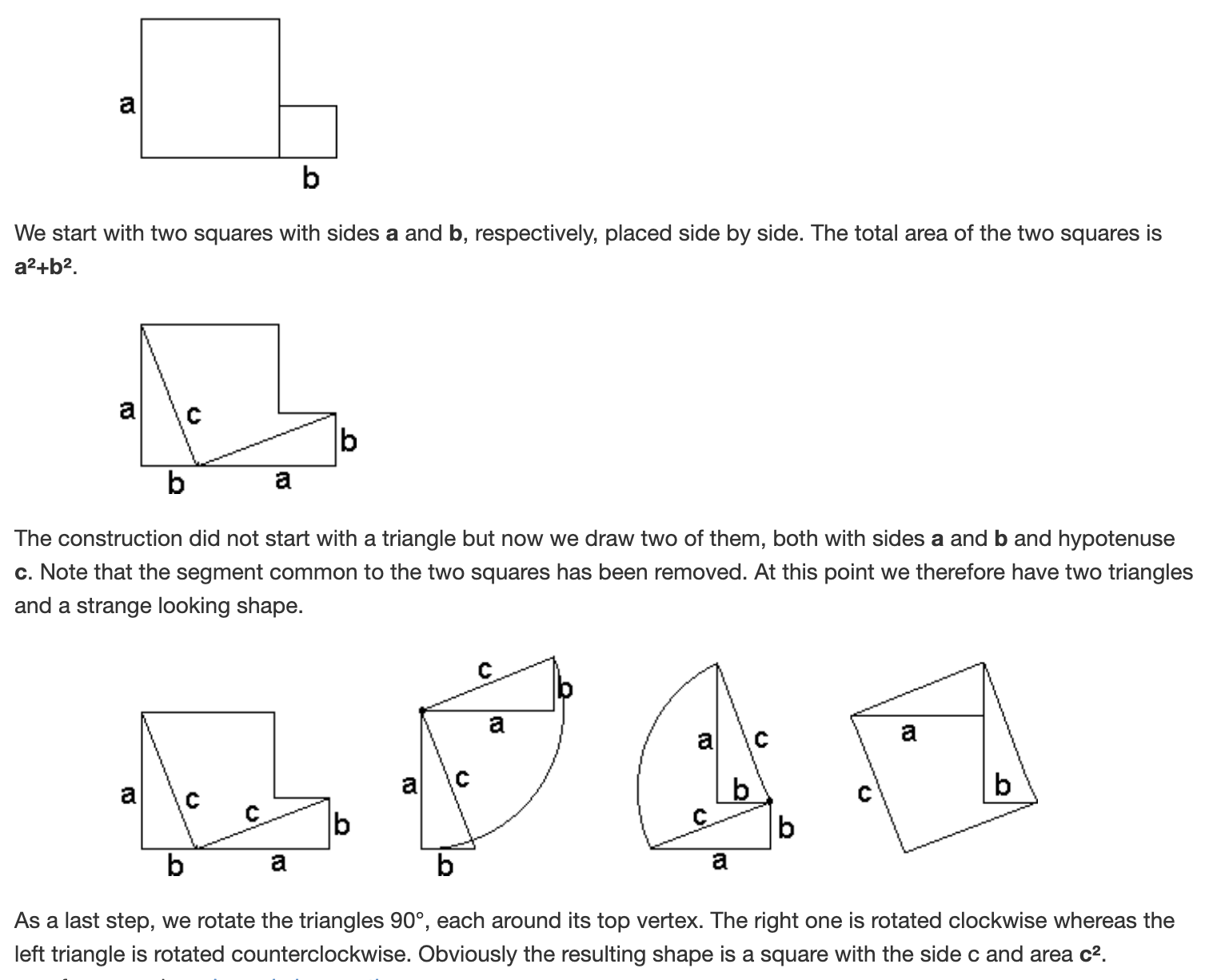
Prove that the final shape shown here is a square, using what we have learned (the Postulates and Propositions).
Problem Set II
Exercise 7 (The Square Root of 3) Read carefully the geometric proof of Theorem thm-sqrt2-irrational, which proves \(\sqrt{2}\) is irrational by showing its impossible to make two integer side-length squares where one has twice the area of the other.
Construct a similar argument showing that it is impossible to find two integer side-length equilateral triangles where one has three times the area of the other.
Hint: try to mimic the argument in the book, but now use the diagram below for inspiration
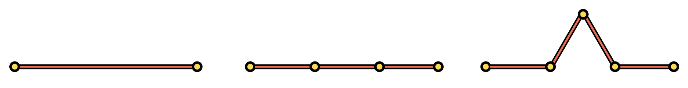
Exercise 8 (Convergence to the Diagonal) Consider a simpler analog of Archimedes’ situation, where instead of trying to measure a curve using straight lines, we are trying to measure a straight diagonal line using only horizontal and vertical segments. The following sequence of paths converges pointwise to the diagonal of the square, but what happens to the lengths?
If you believed that because this sequence of curves limits to the diagonal, its sequence of lengths must limit to the length of the diagonal, what would you have conjectured the pythagorean theorem to be?
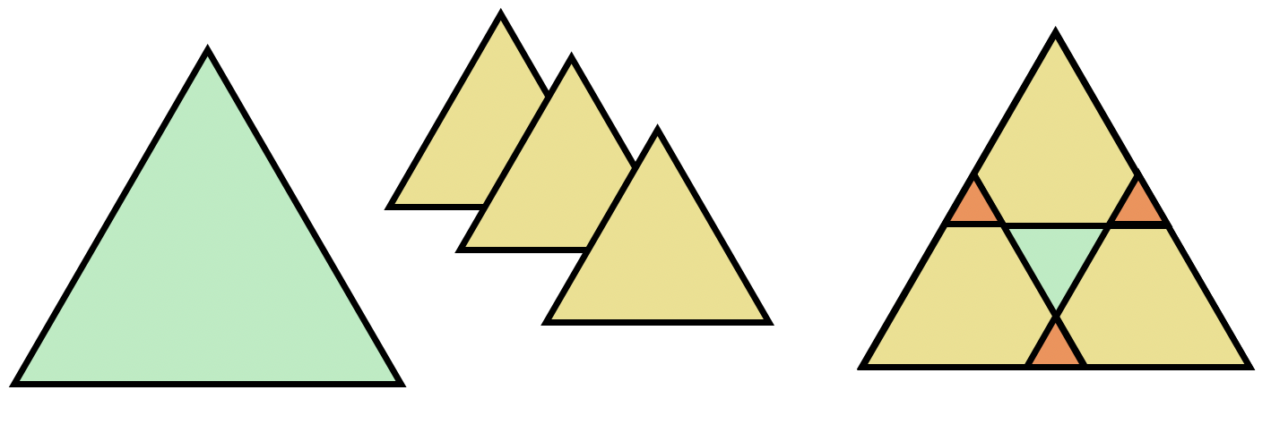
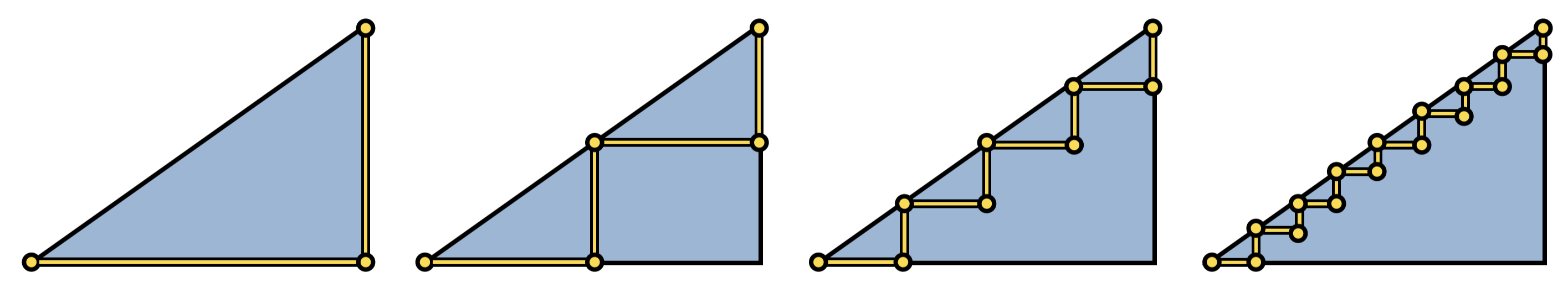
Exercise 9 Use the result of last week’s problem Exercise Inscribing an Equilateral Triangle (that you can inscribe an equilateral triangle with half the side lengths) to produce an alternative proof of Archimedes sum \[\sum_{n=0}^\infty\left(\frac{1}{4}\right)^n=\frac{4}{3}\] By dividing up a triangle instead of a square. Draw some nice pictures (its pretty!)
Exercise 10 Construct an argument in the same spirit as Archimedes’ geometric series to show the following equality: \[\sum_{n=1}^\infty \left(\frac{1}{3}\right)^n=\frac{1}{2}\] Can you cut something iteratively into thirds? It may not be as pretty as Archimedes’, but thats ok!
Fractals
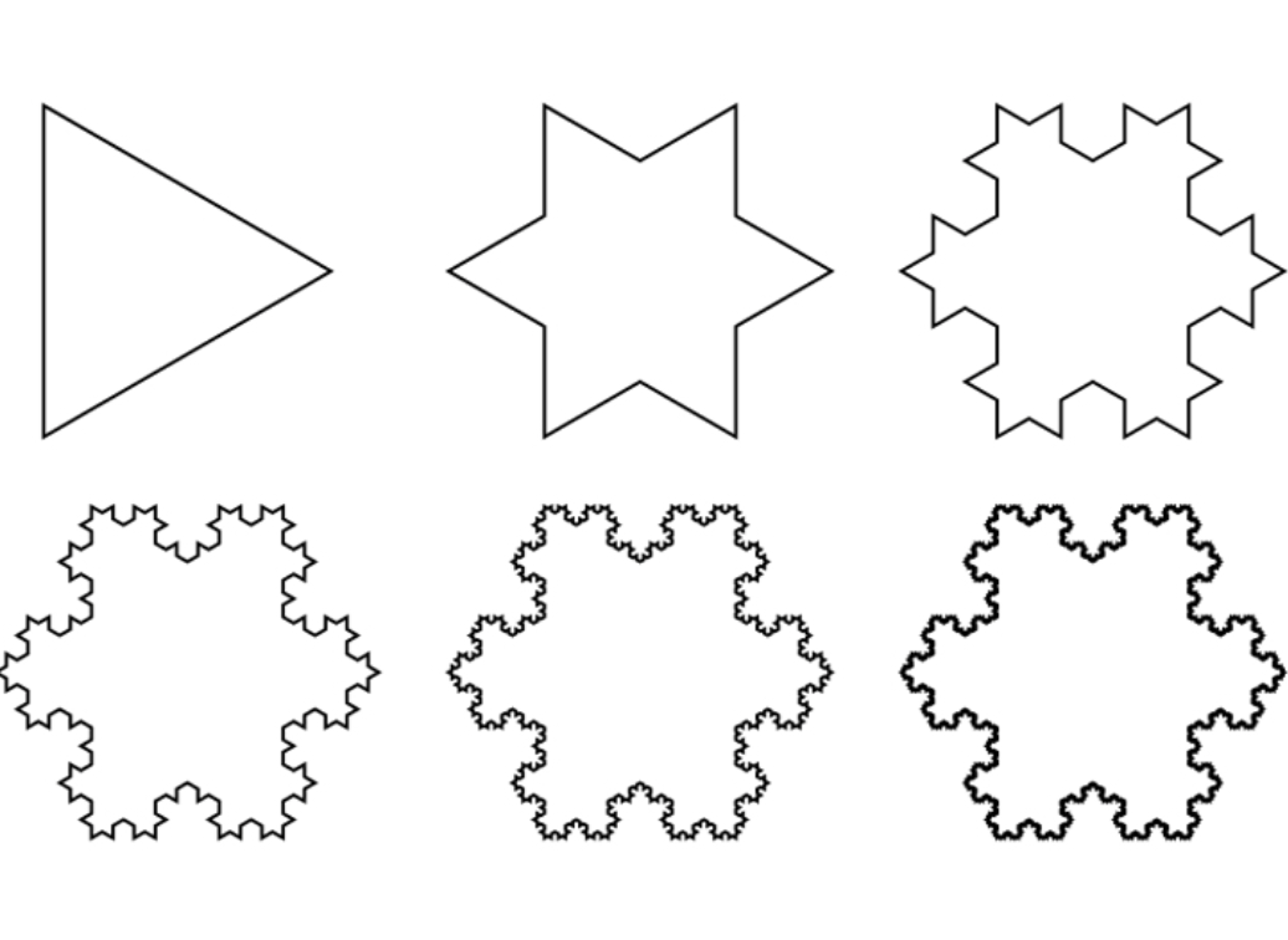
The final two problems involve the Koch Snowflake fractal. In these problems you should still explain why things you are doing are valid geometrically, but you do not need to prove every thing you do from the axioms. We are getting ourselves ready for a calculus mindset!
This shape is the limit of an infinite process, starting at level \(0\) with a single equilateral triangle. To go from one level to the next, every line segment of the previous level is divided into thirds, and the middle third replaced with the other two sides of an equilateral triangle built on that side.
Doing this to every line segment quickly turns the triangle into a spiky snowflake like shape, hence the name. Denote by \(K_n\) the result of the \(n^{th}\) level of this procedure.
Say the initial triangle at level \(0\) has perimeter \(P\), and area \(A\). Then we can define the numbers \(P_n\) to be the perimeter of the \(n^{th}\) level, and \(A_n\) to be the area of the \(n^{th}\) level..
Exercise 11 (The Koch Snowflake Length) What are the perimeters \(P_1,P_2\) and \(P_3\)? Conjecture (and prove by induction, if you’ve had an intro-to-proofs class) a formula for the perimeter \(P_n\).
Explain why as \(n\to\infty\) this diverges (using the type of reasoning you would give in a calculus course): thus, the Koch snowflake fractal cannot be assigned a length!
Before doing the next problem: ask yourself what happens to the area of an equilateral triangle when you shrink its sides by a factor of 3? Can you draw a diagram (similar to that from last week’s Exercise Inscribing an Equilateral Triangle but larger) to see what the ratio of areas must be?
Exercise 12 (The Koch Snowflake Area) What are the areas \(A_1,A_2\) and \(A_3\) in terms of the original area \(A\)?
Find an infinite series that represents the area of the \(n^{th}\) stage \(A_n\) (if you’ve taken an intro to proofs class or beyond - prove it by induction!). Use calculus reasoning to sum this series and show that while the Koch snowflake does not have a perimeter, it does have a finite area!
Problem Set III
Linear Transformations
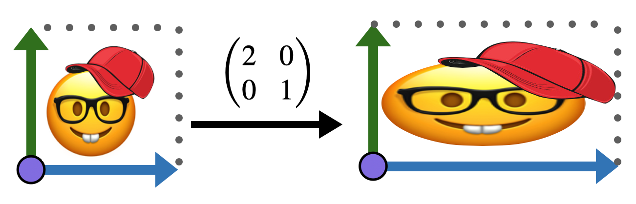
This exercise goes with similar examples in the text, on visualizing linear transformations action on the plane by what they do to the points of the unit square. For instance, we saw that the transformation \(\smat{2&0\\0&1}\) scales the \(x\) axis by a factor of \(2\) and leaves the \(y\) axis invariant, so it performs the following stretch to our little smiley face
Exercise 13 Choose your own image on the plane (hand-drawn is great!), and draw a reference image of it undistorted, inside the unit square. Then draw its image under each of the following linear transformations:
\[\pmat{2&0\\ 0&2}\hspace{1cm} \pmat{1&1\\ 0&1}\hspace{1cm} \pmat{2&1\\ 1&1}\hspace{1cm} \pmat{0&-1\\1 &0}\]
Determinants & Area
Recall the following definition: the determinant of a linear transformation \(M=\left(\begin{smallmatrix}a&b\\c&d\end{smallmatrix}\right)\) is
\[\det M = \left|\begin{matrix}a &b\\c&d\end{matrix}\right| = ad-bc\]
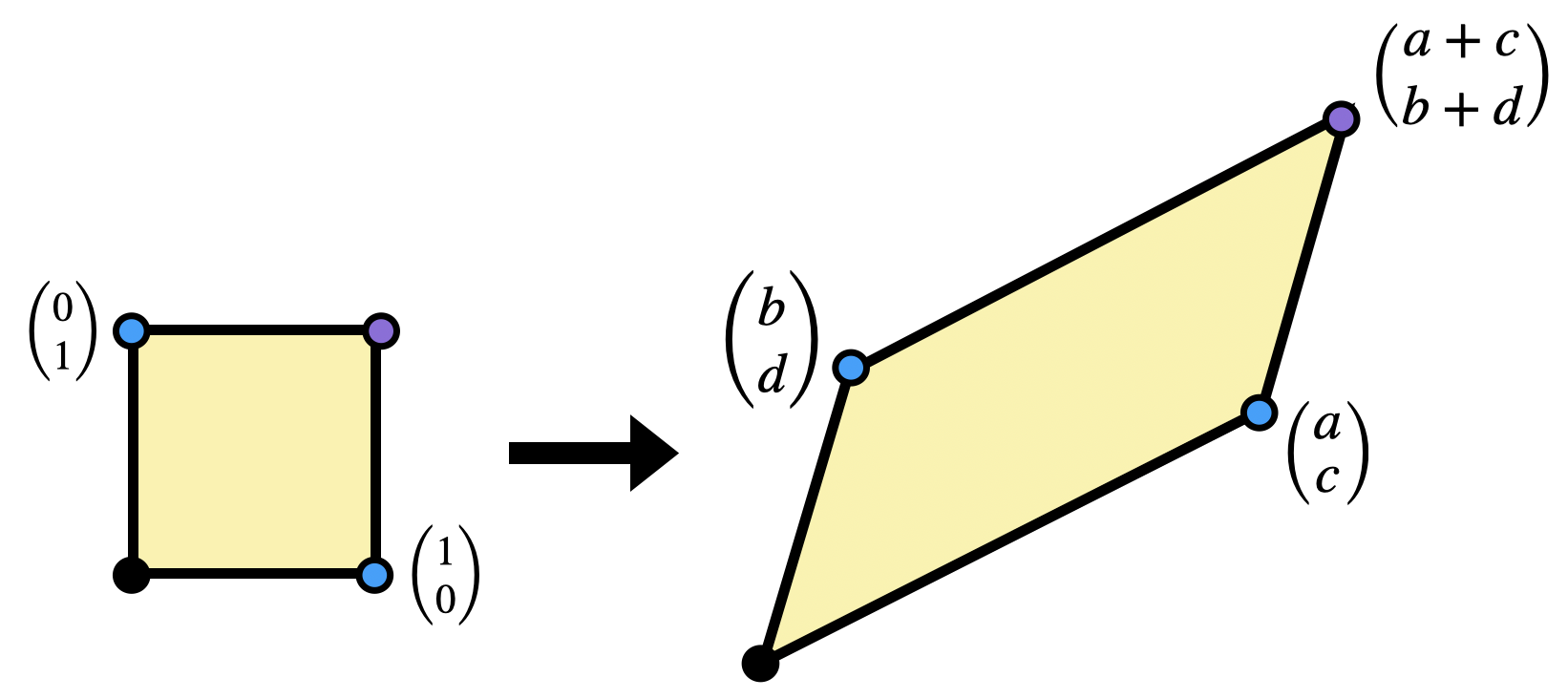
In class, said this measured the area change of the unit square under the linear transformation \(M\), but now we will confirm it. We can actually find this area in a pretty satisfying way using just what we’ve proven about Euclidean geometry so far. We know the areas of squares, rectangles, and right triangles, so let’s try to write the area we are after as a difference of things we know:
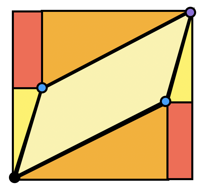
Exercise 14 Show the area of the parallelogram spanned by \(\langle a,c\rangle\) and \(\langle b,d\rangle\) is \(ad-bc\), using the Euclidean geometry we have done, and the diagram above.
Calculating Derivatives
Practice calculating the derivative of multivariate functions as matrices, and applying them to vectors. No proofs, here, just some computations!
Exercise 15 Find the derivatives of the following functions, at the specified points.
- The function \(f(x,y)=(xy,x+y)\) at the point \(p=(1,2)\).
- The function \(\phi(x,y)=\left(xy^2-3x,\frac{x}{y^2+1}\right)\) at the point \(q=(3,0)\).
Now use these to compute the following quantities:
- \(Df_{(1,2)}\langle 3,4\rangle\)
- \(D\phi_{(3,0)}\langle a,b\rangle\)
Differentiating Compositions
This is another problem which focuses on the new computational skills, using linear algebra. No proofs here either!
Exercise 16 If \(F,G,H\) are the following multivariate functions \[F(x,y)=(x-y,xy)\] \[G(x,y)=(-y,x)\] \[H(x,y)=(x^3,y^3)\]
Differentiate the following compositions:
- \(F\circ G\) at \((1,1)\)
- \(G\circ G\) at \((0,2)\)
- \(F\circ G\circ H\) at \((-1,3)\).
When the Derivative is Constant
In class, we proved that if a function is linear, then its derivative is constant. But is this the only time a function’s derivative is constant? Certainly no - the derivative of \((x,y)\mapsto(x+1,y)\) is constant (equal to the identity matrix!), even though this function is not linear.
We call a function affine if it is the composition of a linear function and addition of a constant. For instance, \(2x+3\) or \(5x+2y-7\) are affine functions. We call a multivariable function affine if each of its component functions is affine.
Exercise 17 (When the derivative is constant) Prove that a function \(\phi\colon\RR^2\to\RR^2\) has a constant derivative if and only if the function is affine: that is, a linear map plus constants.
Hint: if the derivative is a constant matrix, can you integrate each entry (with respect to the right variable) to figure out what the original functions were?
Problem Set IV
Parameterization Invariance
Below are four different curves which all trace out the same set of points in the plane: the segment of the \(x\) axis between \(0\) and \(4\).
\[\alpha(t)=(t,0)\hspace{1cm}t\in[0,4]\] \[\beta(t)=(2t,0)\hspace{1cm}t\in[0,2]\] \[\gamma(t)=(t^2,0)\hspace{1cm}t\in[0,2]\]
Because these all describe the same set of points, we of course want them to have the same length! But our definition of the length function involves integrating infinitesimal arclengths (derivatives), and these curves don’t all have the same derivative! Thus, to really make sure our definition makes sense, we need to check that it doesn’t matter which parameterization we use, we will always get the same length.
Exercise 18 Check these three parameterizations of the segment of the \(x\)-axis from \(0\) to \(4\) all have the same length.
After doing this exercise, read the proof of Theorem Length & Parameterization Invariance (which follows this exercises’ original location in the text): you don’t have to write anything here, but it’s good to see how do to this in general with the chain rule!
Non-Isometries
Exercise 19 Write down a linear map that sends both \(\langle 1,0\rangle\) and \(\langle 0,1\rangle\) to unit vectors, but is not an isometry.
This shows there’s not a shortcut to checking something is an isometry by just seeing what happens to the basis vectors!
Composition and Inversion of Isometries
Exercise 20 If \(\phi\) and \(\psi\) are two isometries of \(\EE^2\), prove that both the composition \(\phi\circ\psi\) is an isometry, and the inverse \(\phi^{-1}\) is an isometry.
Remember, you will need to explain why at every point \(p\in \EE^2\), these maps do not change the lengths of tangent vectors. This will probably involve the multivariable chain rule, whether you do it in words, or in equations!
Homogenity and Isotropy
In class we built a couple different sorts of isometries from the basic ones we constructed by hand (translations and rotations about 0). In this exercise, you are to prove the existence of another very useful isometry. We will use this homework problem all the time
Exercise 21 (Moving from \(p\) to \(q\).) Given any two pairs \(p,v_p\) and \(q,w_q\) of points \(p,q\) in Euclidean space and unit tangent vectors \(v_p\in T_p\EE^2\), \(w_q\in T_q \EE^2\) based at them, prove that there exists an isometry taking \(v_p\) to \(w_q\).
Hint: try to combine pieces we know about, and prove the result does what you need by applying it both to the point \(p\), and applying its derivative to the vector \(v\).
Lines of Symmetry
In this exercise we will investigate the third potential definition of line, which involves isometries.
Definition 1 (Line of Symmetry) A fixed point of an isometry \(\phi\colon \EE^2\to\EE^2\) is a point \(p\) with \(\phi(p)=p\).
A curve \(\gamma\) is called a line of symmetry of \(\EE^2\) if there exists an isometry which fixes \(\gamma(t)\) for all \(t\).
In this exercise, you show that the curves which are lines of symmetry are exactly the same as the curves which are lines under Archimedes’ definition!
Exercise 22 (Reflections in Any Line)
Show that map \(\phi(x,y)=(x,-y)\) is an isometry of \(\EE^2\). Explain why this shows that the \(x\)-axis is a line of symmetry of the plane.
Show that every curve which is distance-minimizing in the plane is also a line of symmetry. Hint: given an isometry that reflects in the \(x\) axis, can you build an isometry that reflects in any other line? Consider moving the line to the \(x\) axis, reflecting, and then moving back.
Equilateral Triangles Revisited
In this question we will revisit two problems from Greek geometry. That is we will be re-proving things we knew before, so we know they are still true in our new foundations!
This problem requires the distance function on the Euclidean plane, which we did not get to in class on Thursday, but will cover on Tuesday. However - you all areadly know the distance function so you can absolutely complete the homework now if you like!
Definition 2 If \(p=(x,y)\) and \(q=(a,b)\) are two points in the Euclidean plane, the distance from \(p\) to \(q\) is the length of the shortest curve connecting them. Working this out, we find the familiar pythagorean theorem:
\[\dist(p,q)=\sqrt{(x-a)^2+(y-b)^2}\]
First, we re-prove the very first proposition of Euclid, the existence of an equilateral triangle. Then we redo your earlier homework problem on finding a smaller equilateral triangle inside of it, of half the side lengths (but this is much easier with our new tools!).
Exercise 23
Beginning with the segment \([0,\ell]\) along the \(x\)-axis, construct an equilateral triangle by finding the coordinates of a point \(p=(x,y)\in\EE^2\) which is equidistant from both endpoints of the segment.
Re-prove that inside of this equilateral triangle, you can inscribe a smaller one with exactly half the side length. Hint: just find where the vertices should be, and then measure the distances between them!
Length of a Parabola
Arclength integrals give a good opportunity to practice a lot of Calculus II integration techniques. Even for relatively simple curves like the parabola, the answers can be quite nontrivial!
Exercise 24 (The Length of a Parabola) Find the length of the parabola \(y=x^2\) between from \(x=0\) to \(x=a\), following the steps below.
- Paramterize the curve as \(c(t)=(t,t^2)\), show the arclength integral is \(L(a)=\int_{[0,a]}\sqrt{1+4t^2}\)
- Perform the trigonometric substitution \(x=\frac{1}{2}\tan\theta\) to convert this to some multiple of the integral of \(\sec^3(\theta)\).
- Let \(I=\int\sec^3(\theta)d\theta\) and do integration by parts with \(u=\sec\theta\) and \(dv=\sec^2\theta\).
- After parts, use the trigonometric identity \(\tan^2\theta=\sec^2\theta-1\) in the resulting integral to get another copy of \(I=\int\sec^3\theta d\theta\) to appear.
- Get both copies of \(I\) to the same side of the equation and solve for it! To check your work at this stage, you should have found that \[\int\sec^3\theta d\theta = \frac{1}{2}\sec\theta\tan\theta+\frac{1}{2}\ln\left|\sec\theta+\tan\theta\right|\]
- Relate this back to your original integral, and undo the substitution \(x=\frac{1}{2}\tan\theta\): can you use somet trigonometry to figure out what \(\sec\theta\) is?
- Finally, you have the antiderivative in terms of \(x\)! Now evaluate from \(0\) to \(a\).
Minimizing a Function by Minimizing its Square
Here’s a problem that’s straight up single variable calculus, but turns out to be a quite useful “trick” in geometry! Oftentimes we want to minimize a function in geometry (like arclength, or distance) but this turns out to be technically hard because of the square root. One might wonder - what happens if I square the function, and try to minimize that instead? That will have an easier formula (no roots), but will I get the right answer?
This exercise shows, yes you will!
Exercise 25 (Minimizing the Square: A Very Useful Trick!) Let \(f(x)\) be a differentiable positive function of one variable, and let \(s(x)=f(x)^2\) be its square. Show that the minima of \(s(x)\) and \(f(x)\) occur at the same points, by following the steps below:
First, assume \(x=a\) is the location of a minimum of \(f\). What does the first and second derivative test tell you about the values \(f^\prime(a)\) and \(f^{\prime\prime}(a)\)? Use this, together with the fact that \(f(a)>0\) to show that \(x=a\) is also the location of a minimum of \(s\) (using the second derivative test).
Conversely, assume \(x=a\) is the location of a minimum of \(s(x)\). Now, you know information about the derivatives \(s^\prime(a)\) and \(s^{\prime\prime}(a)\). Use this to conclude information about \(f^\prime(a)\) and \(f^{\prime\prime}(a)\) to show that \(a\) is a minimum for \(f\) as well.
Problem Set V
The Parallel Postulate
Recall that Playfair’s Axioms (already suggested by Proclus in the 400s) was a simpler re-phrasing of Euclid’s original fifth postulate on parallel (that is, nonintersecting) lines.
Proposition 1 Given any line \(L\) in \(\EE^2\), and any point \(p\in \EE^2\) not lying on \(L\), there exists a unique line \(\Lambda\) through \(p\) which does not intersect \(p\).
Exercise 26 Prove Proposition prp-proving-playfairs-axiom.
Hint: use isometries to help you out!
First, use an isometry to move \(L\) to the \(x\)-axis. Then, use another isometry to keep \(L\) on the \(x\) axis, but to move \(p\) to some point along the \(y\) axis. Then, prove that through any point on the \(y\) axis there is a unique line that does not intersect the \(x\)-axis.
Similarities and Lines
We saw in Theorem Isometries Send Lines to Lines that any isometry will carry a line to another line. The same is true more generally of similarities:
Exercise 27 (Similarities Send Lines to Lines) Let \(\gamma\colon\RR\to\EE^2\) be a line, and \(\sigma\colon\EE^2\to\EE^2\) be a similarity. Prove that \(\sigma\circ\gamma\) is also a line.
*Hint-replicate the proof of Theorem Isometries Send Lines to Lines as closely as possible, replacing the isometry \(\phi\) with the similarity \(\sigma\), and keeping track of the scaling factors of \(\sigma\) versus \(\sigma^{-1}\) (Proposition prp-similarity-scaling-inverse).
Distance to a Line.
In this problem it’s probably helpful to use the ‘calculus trick’ offered as an optional problem last week: that is, if you are looking to minimize a positive function \(f(x)\), you can instead try to minimize the function \(f(x)^2\), and you’ll find the same \(x\)-value achieves the minimum.
The reason this is useful to us is that the distance function in geometry has a square root in it, and differentiating roots can be a lot of work. So this says instead we can minimize the square of distance to find the right point.
Exercise 28 (Closest Point on Line) Let \(L\) be the line traced by the affine curve \(\gamma(t)=\pmat{a t+ c\\ bt +d}\), and \(O\) be the origin.
Alternatively, do this for the line \((2t+1,3t-4)\), to save yourself a lot of \(abcd's\).
- Find the point \(p\in L\) which is closest to \(O\).
- Calculate \(\dist(O,L)\).
- What angle does the segment connecting \(p\) to \(O\) make with the line \(L\)? (We haven’t reviewed the definition of angle yet, so just use your knowledge of angles from precalculus: pick a line an compute an example!)
This problem shows how we can use calculus as a tool to discover a geometric fact: here we learned something about where the closest point on a line is located (by finding it with calculus, then calculating the angle formed).
Often calculus can provide the tools needed for discovery of a new fact, but once its known, one can often go back and find a geometric (more in the style of Euclid) proof that all of a sudden makes the conclusion feel inevitable.
Exercise 29 (Closest Point: Geometric Reasoning) Now that we know the answer, formulate in your own words a geometric proposition that describes which point \(p\) on a line is closer to a given point \(q\) not on that line.
Prove this propostion without just taking a derivative, try to reason more like the Greeks, using other facts and theorems that we’ve proven.
Hint: if you pick some other point \(r\) along \(L\), can you draw a triangle using \(p,q,r\)? How can we use the geometry of this triangle to show that \(r\) is farther from \(q\) than \(p\) was? Does the Pythagorean theorem say anything useful?
Intersecting Circles
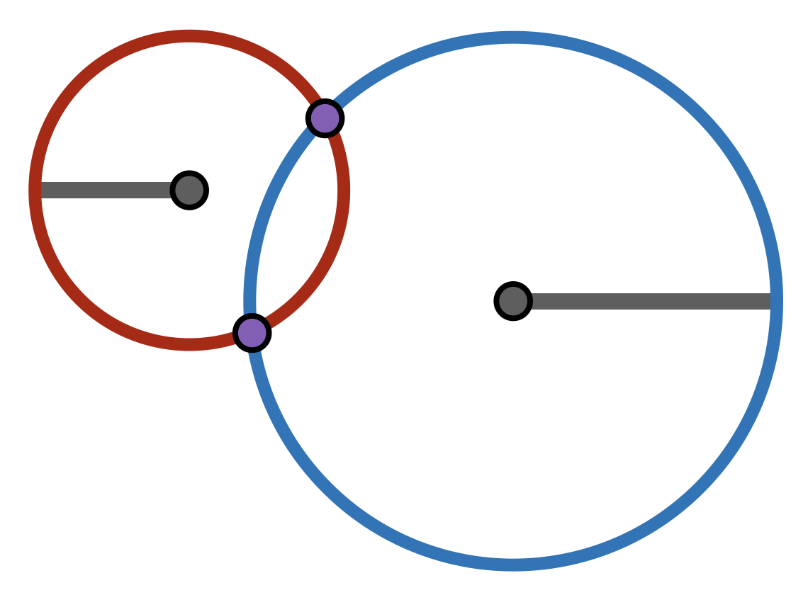
Recall that in all of Euclid’s axioms, conditions for intersections with circles were never specified! Indeed - Euclid intersected two circles in his construction of the equilateral triangle. Now that we have a precise description of circles in our new foundations, we can fix this gap:
Exercise 30 Prove that two circles intersect each other if the distance between their centers is less than or equal to the sum of their radii.
Alternatively: do this for the specific case where the circles radii are 3 and 4, and the distance between thier centers is 5.
Hint: start by applying an isometry to move one of the circles to have center \((0,0)\), and then another isometry to rotate everything so the second circle has center \((x,0)\) along the \(x\)-axis. This will make computations easier!
Parabolas
A parabola was one of few curves that the Greeks understood. However, while we often think of a parabola algebraically that was not their original definition!
Definition 3 (Parabola) Given a point \(f\) (called the focus) and a line \(L\) not containing \(f\) (called the directrix), the parabola with focus \(f\) and directrix \(L\) is the curve \(C\) of points where for each \(p\in C\) the distance to the focus equals the distance to the line: \[\dist(p,f)=\dist(p,L)\]
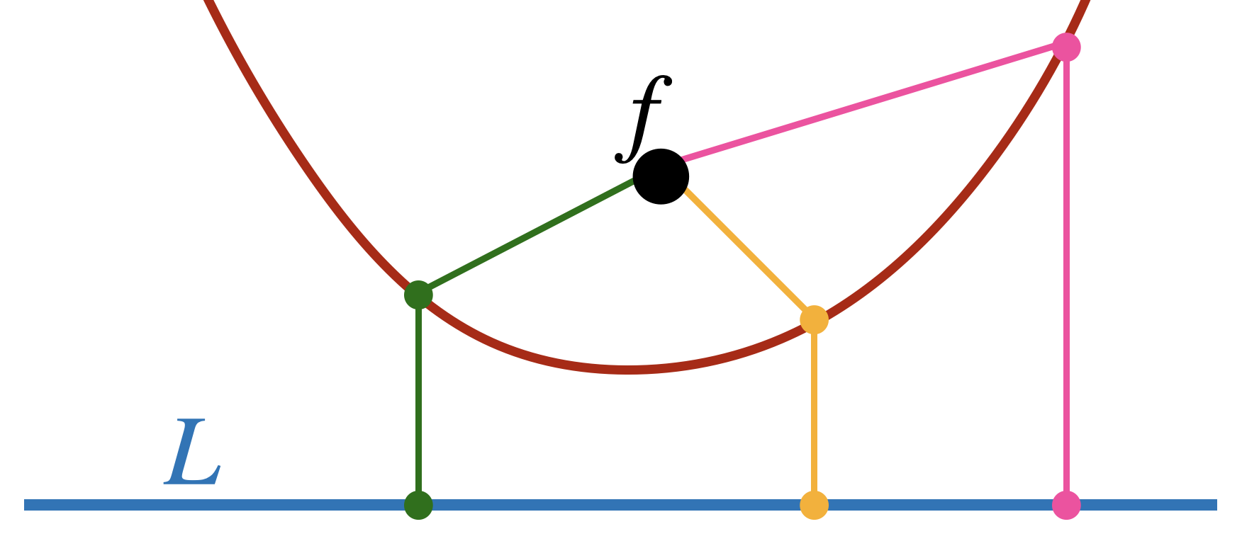
Exercise 31 In this problem we confirm that \(y=x^2\) is indeed a parabola! Let \(L\) be a horizontal line intersecting the \(y-\)axis at some point \((0,-\ell)\), and \(f=(0,h)\) be a point along the \(y\)-axis for \(\ell,h>0\).
- Write down an algebraic equation for the coordinates of a point \((x,y)\) determining when it is on the parabola with focus \(f\) and directrix \(L\).
- Find which point \(f\) and line \(L\) make this parabola have the algebraic equation \(y=x^2\).
Problem Set VI
Right Angles
In this set of two problems, we make use of the fact that we can finally measure angles rigorously in our new geometry, to reprove an important fact we already know, and to prove the one remaining postulate of Euclid: the 4th.
Exercise 32 Prove that rectangles exist, using all of our new tools! (Ie write down what you know to be a rectangle, explain why each side is a line segment, parameterize it to find the tangent vectors at the vertices, and use the dot product to confirm that they are all right angles).
To prove Euclid’s 4th postulate, we need to first phrase it more precisely than Euclid’s original all right angles are equal.
Proposition 2 (Euclids’ Postulate 4) Given the following two configurations:
- A point \(p\), and two orthogonal unit vectors \(u_p,v_p\) based at \(p\)
- A point \(q\), and two orthogonal unit vectors \(a_q,b_q\) based at \(q\)
There is an isometry \(\phi\) of \(\EE^2\) which takes \(p\) to \(q\), takes \(u_p\) to \(a_q\), and \(v_p\) to \(b_q\).
Exercise 33 Prove Euclids’ forth postulate holds in the geometry we have built founded on calculus.
Hint: there’s a couple natural approaches here.
- You could directly use Exercise Moving from p to q. from a previous homework to move one point to the other and line up one of the tangent vectors. Then deal with the second one: can you explain why its either already lined up, or will be after one reflection?
- Alternatively, you could show that every right angle can be moved to the “standard right angle” formed by \(\langle 1,0\rangle, \langle 0,1\rangle\) at \(O\). Then use this to move every angle to every other, transiting through \(O\)
Measurement of the Circle
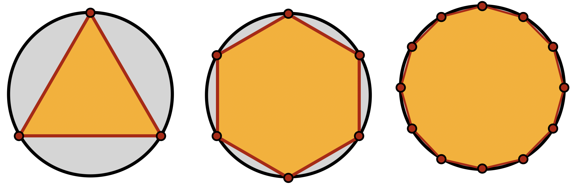
The half angle identities played a crucial role in Archimedes’ ability to compute the preimeter of \(n\) gons in his paper The Measurement of the Circle. Indeed, to calculate the circumference of an inscribed \(n\)-gon, its enough to be able to find \(\sin\tau/(2n)\):
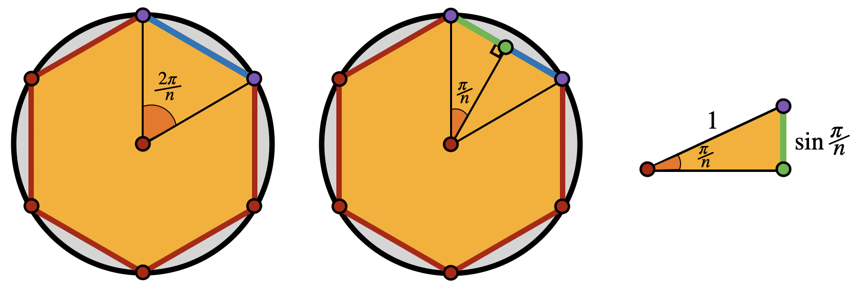
By repeatedly bisecting the sides, we can start with something we can directly compute - like a triangle, and repeatedly bisect to compute larger and larger \(n\)-gons.
In the book, I use the half-angle identities to compute the exact value of \(\sin\tau/12\). Follow that example further, to retrace the steps of Archimedes.
Exercise 34 Continue to bisections until you can compute \(\sin(\tau/(2\cdot 96))\). What is the perimeter of the regular \(96\)-gon (use a computer to get a decimal approximation, after your exact answer).
Explain how we know that this is provably an underestimate of the true length, using the definition of line segments.
Optional: Be brave - and go beyond Archimedes! Compute the circumference of the 192-gon.
Quadrature of the Parabola
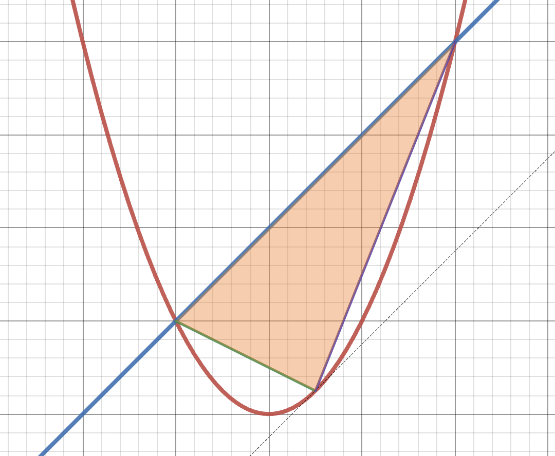
This is also a two-problem series, where we complete Archimedes famous Quadrature of the Parabola using modern tools from calculus. Archimedes problem was about a parabolic segment: that is, the region enclosed by a parabola and a line segment connecting two points on the parabola. Instead of working in complete generality like Archimedes, we will be content to just study a special case in this problem. We will look at the parabola \(y=x^2\), and the parabolic segment cut out by this and the line connecting \((-1,1)\) to \((2,4)\).
Recall Archimedes main result: the area of this parabolic segment is \(4/3\)rds the area of the largest inscribed triangle, which is the triangle whose base is the line segment, and third vertex lies on the parabola at the point where the tangent line is parallel to the base.
Exercise 35
- Write down a formula for the area of the triangle whose third vertex lies at \((x,x^2)\)
Hint: instead of finding the height of the triangle to use \(\tfrac{1}{2}bh\), can you use the fact that the determinant of a matrix calculates the area of a parallelogram whose sides are the column vectors, and that the area of a the triangle you want is half a parallelogram?
- Use Calculus I to find the point \(x\) where the inscribed triangle has maximal area. Then show that Archimedes was right: the slope of the tangent line to the parabola at this point is exactly the same as the slope of the line segment forming the triangle’s base!
This gives us the starting point: the area for which archimedes wishes to compare the parabolic segment. Next - we need to find the parabolic segment’s area. We could of course follow Archimedes’ original method (and if you choose to, this can be your class project!) But here, we will use our modern tools and confirm the answer with calculus:
Exercise 36 Compute the area of the parabolic segment (via integration, as the area between two curves). Show that its exactly \(4/3\)rds the area of the triangle!
The Area and Circumference Constants
A circle has a circumference constant: the ratio of its radius to its circumference, which we’ve named \(\tau\). But it also has an *area constant: the ratio of its area to the square of its radius, which we’ve named \(\pi\).
It was Archimedes who first showed that these two constants were intimately related, by finding that \(\tau = 2\pi\). Here we will again use our modern tools to reprove Archimede’s result.
Tau is the circumference of the unit circle \(x^2+y^2=1\). We can parameterize the top half of this circle via \[\gamma(t)=(t,\sqrt{1-t^2})\]
And then compute its arclength via the integral \[\frac{\tau}{2}=\int_{-1}^1 \|\gamma^\prime(t)\|dt=\int_{-1}^1\frac{1}{\sqrt{1-t^2}}dt\]
But we can also write down the area of the circle as an integral: the top half of the circle is \(y=\sqrt{1-x^2}\) and the bottom half is \(y=-\sqrt{1-x^2}\) so the area is
\[\pi = \int_{-1}^1\int_{-\sqrt{1-x^2}}^{\sqrt{1-x^2}}dydx=\int_{-1}^1 2\sqrt{1-x^2}dx\]
Your goal in this problem is to show these two integrals are equal to one another!
Exercise 37 Prove that \[\int_{-1}^1\frac{1}{\sqrt{1-t^2}}dt=\int_{-1}^1 2\sqrt{1-x^2}dx\] Thus showing that \(\frac{\tau}{2}=\pi\).
Hint: Do \(u\)-substitutions to the integrals to make them into the same integral. The goal isn’t to evaluate them and get a number! This is just a Calc II problem - but a tricky one, so here’s one outline you could follow:
Rewrite the area integrand \(\sqrt{1-x^2}\) as \(\frac{1-x^2}{\sqrt{1-x^2}}\). Use properties of integrals to break this into two integrals, and see \[\pi = \tau -\int_{-1}^1\frac{2x^2}{\sqrt{1-x^2}}dx\]
Now we just have to evaluate this new integral: Do the \(u\)-substitution \(u=\sqrt{1-x^2}\) to this, to show that \[\int_{-1}^1 \frac{2x^2}{\sqrt{1-x^2}}dx=\int_{-1}^1 2\sqrt{1-u^2}du=\pi\] (This \(u\)-sub requires some work: you’ll need at some point to solve for \(x\) in terms of \(u\)!)
Now just assemble the pieces! You never completed a single integral, but you still managed to prove that \(\tau =2\pi\).
Problem Set VII
Trigonometric Identities:
The following exercise has you compute with some trigonometric identities, which we needed to find the volume of spheres:
Exercise 38 (Integrating \(\cos^4(\theta)\)) Start with the angle sum-identity we derived in class some lectures back \[\cos(a+b)=\cos(a)\cos(b)-\sin(a)\sin(b)\]
Use this to derive an identity relating \(\cos(2\theta)\) to \(\cos^2(\theta)\) (we did most of this in class - but repeat it for yourselves). Now use this identity twice to show
\[\cos^4(\theta)= \frac{3}{8}+\frac{\cos 2\theta}{2}+\frac{\cos 4\theta}{8}\]
by writing \(\cos^4\theta = (\cos^2\theta)^2\). Then use this to confirm that
\[\int_0^{\frac\tau 4}\cos^4\theta = \frac{3}{8}\frac{\tau}{4}\]
This result was crucial to our calculation of the volume of the four dimensional sphere in class, where we showed (via a trigonometric substitution)
\[\mathrm{vol}=\frac{8\pi}{3}\int_0^{\tau/4}\cos^4(\theta)d\theta\]
Using this result gave us the final answer:
\[\begin{align*} \mathrm{vol}&=\frac{8\pi}{3}\frac{3}{8}\frac{\tau}{4}\\ &= \frac{\pi\tau}{4}\\ &=\frac{\pi^2}{2} \end{align*}\]
The 5-Dimensional Sphere
The unit sphere in five dimensions is given by the set of points \((x,y,z,w,u)\) satisfying \[x^2+y^2+z^2+w^2+u^2=1\]
Exercise 39 Calculate the volume of this space by slicing along the \(u\) direction. Show that the slices are four dimensional spheres: what’s the radius? Use the volume formula in four dimensions we derived in class \[\mathrm{vol}(r)=\frac{\pi^2}{2}r^4\] to write down the volume of each slice, and then perform the integral to confirm that the 5-dimensional volume is \[\frac{8\pi^2}{15}\]
(This will not need any trigonometric substitution) Once you have this, find the “surface area” of this 5-dimensional sphere by differentiation.
High Dimensional Spheres and Cylinders
Exercise 40 The discovery Archimedes was most proud of was that the surface area of the sphere in 3-dimensions was the same as the area of the smallest cylinder surrounding it.
Is the same true in four dimensions? (A four-dimensional cylinder has a sphere’s surface as its “base”, just like a three dimensional cylinder has a circle’s length as its base!)
Problem Set VIII
The Dot Product
One thing we used in our arguments building up the basics of spherical geometry was the fact that the dot product has a nice derivative rule.
Exercise 41 (Product Rule for Dot Product) Let \(f(t)=\langle f_1(t),f_2(t),f_3(t)\rangle\) and \(g(t)=\langle g_1(t),g_2(t),g_3(t)\rangle\) be two vector functions. Prove that the dot product satisifes the product rule: \[\frac{d}{dt}\left(f(t)\cdot g(t)\right)= f^\prime(t)\cdot g(t)+f(t)\cdot g^\prime(t)\]
Our use of the dot product overall is as a tool to give the sphere geometry it defines what we mean by infinitesimal length and by angle. Often we will use this just as a theoretical tool - but its good to get some hands-on practice at the beginning, measuring some actual angles.
Exercise 42 Consider the curves \(\alpha(t)=(\cos t,\sin t,0)\) (the equator of the sphere), and \(\beta(t)=(0,\sin(t),\cos(t))\) (a line of longitude). Prove that they
- Intersect each other at the \(t=\pi/2\)
- Form a right angle at their point of intersection.
Draw a picture of this situation in 3D on a sphere.
Isometries
Recall the definition of an isometry of \(\SS^2\) is a function \(\phi\colon\SS^2\to\SS^2\) which preserves the dot product (or equivalently, preserves infinitesimal lengths).
Exercise 43 A permutation matrix is a square matrix where every row and column has exactly one “1”, and the other entries are zero. Prove the following permutation matrix \[A=\pmat{0&1&0\\1&0&0\\0&0&1}\]
can be used to define an isometry of \(\SS^2\) by the formula \[\phi(x,y,z)=A\pmat{x\\ y\\ z}\] directly from the definition of isometry.
In class we are working our way to prove some facts about isometries, mimicking what we did in the Euclidean plane. In particular, on Tuesday we will prove the following two important facts.
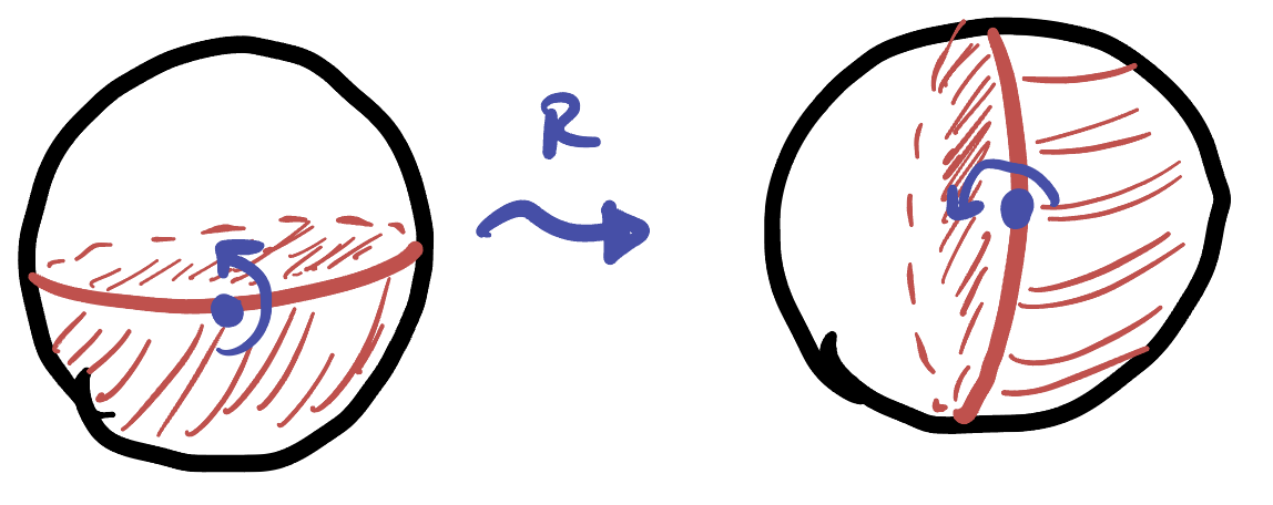
Theorem 1 (The Sphere is Homogeneous) Given any two points \(p\) and \(q\) on the sphere, there is an isometry taking \(p\) to \(q\):
Proposition 3 Let \(N\) be the north pole, and \(v\) be any unit vector in \(T_N\SS^2\). Then there exists an isometry \(\phi\) of the sphere which fixes \(N\) and takes \(\langle 1,0,0\rangle\in T_N\SS^2\) to \(v\).
The first is an analog of translations of the Euclidean plane: we can always find an isometry of the sphere that takes any point to any other. And the second is similar to when we proved that you could build rotations of \(\EE^2\) about the origin (we’ll actually prove it, using that exact theorem!)
Your goal in these next problems is to use these theorems to prove even more: first, prove that you can actually rotate the sphere fixing any point you wish (not just the north pole!)
Exercise 44 Use Proposition prp-sphere-rotate-north-pole and Theorem The Sphere is Homogeneous to show the sphere is isotropic: that given any point \(p\in\SS^2\) and any two unit vectors \(v,w\in T_p\SS^2\), there exists an isometry of \(\SS^2\) fixing \(p\) and taking \(v\) to \(w\).
(Hint: first show you can do this when \(p\) is the north pole! Then use homogenity and a conjugation. Be inspired by the Euclidean proof!)
Next, just like in Euclidean space we often find it useful to combine homogenity and isotropy into one condition: we can move any point and any tangent vector to any other point and tangent vector that we like!
Exercise 45 Let \(p,q\) be any two points on the sphere, and \(v\) a unit tangent vector at \(p\) and \(w\) a unit tangent vector at \(q\). Then there is an isometry of \(\SS^2\) taking \((p,v)\) to \((q,w)\).
Hint: Look back at Ex 4 Homework 4!
Problem Set IX
Acceleration
We saw in class that the acceleration of a curve on the unit sphere is the projection of its \(\EE^3\) acceleration vector onto the tangent plane. In terms of the curve \(\gamma(t)\), that worked out to
\[\acc_\gamma(t)=\gamma^{\prime\prime}(t)-\left(\gamma^{\prime\prime}(t)\cdot\gamma(t)\right)\gamma(t)\]
Exercise 46 (Geodesic Curvature) The magnitude of the acceleration of a unit speed curve is called its geodesic curvature: its a way to measure how much that curve differs from a geodesic. This exercise, you will calculate the geodesic curvature of the circle of radius \(r\) on \(\SS^2\):
- Let \(C\) be a circle on \(\SS^2\) of radius \(r\) (to make calculations easy, let \(C\) be centered at the north pole if you like).
- Write down a parameterization of \(C\) (hint: you know the plane that \(C\) lies in, and its Euclidean radius in that plane!)
- Find a parameterization of \(C\) that has speed \(1\) (hint if you wrote down a parameterization above, what speed does it travel at? Can you adjust it so the new curve has speed \(1\)?)
- What is the acceleration felt on \(\SS^2\) if you go around a circle of radius \(r\) at unit speed? What is it’s magnitude?
The idea of measuring acceleration along a surface in \(\EE^3\) as the projection of the second derivative onto the tangent space is foundational to the study of surfaces beyond just the sphere (it is one of the fundamental concepts in differential geometry). When the acceleration of a curve \(\gamma\) is equal to zero on a surface, then we say that curve is a geodesic on the surface. So, the equations we get by setting the acceleration equal to zero give us a set of differential equations that tell us what the geodesics are! These are called the geodesic equations
In this next problem, we will get a small taste of what happens in differential geometry, when our space is not nice and symmetric like the plane or the sphere, and we have to resort to finding the geodesic equations and solving them (you won’t have to solve them! Just find them….)
Exercise 47 (Geodesics on Surfaces) Let \(S\) be the surface \(z=x^2+y^2\), which is the output of the function \(F\colon\EE^2\to\EE^3\) given by \[F(x,y)=(x,y,x^2+y^2)\in \EE^3\].
Let \(p=F(x,y)\) be a point on \(S\).
- Use calculus to find two tangent vectors to the graph at a point \(p\): Hint: \(DF_{(x,y)}\langle 1,0\rangle\) and…?
- Find a normal vector \(n\) to the graph at \(p\) using these and the cross product.
- Write down the projection of a vector \(v=\langle a,b,c\rangle\) onto the normal vector \(n\).
- Write down the projection of \(v=\langle a,b,c\rangle\) onto the tangent plane \(T_{p} S\).
This is all the data we need to be able to compute acceleration along the surface \(S\)! Let \(\gamma(t)\) be a curve that lies on the surface, so \[\gamma(t)=F(x(t),y(t))=\left(x(t),y(t),x(t)^2+y(t)^2\right)\] for some function \(x(t)\) and \(y(t)\).
- Find \(\gamma^{\prime\prime}\)
- Find the acceleration of \(\gamma\) on the surface \(S\), in terms of \(x(t)\) and \(y(t)\).
- What are the geodesic equations for \(S\)?
Curvature
We saw in class that the circumference of a circle of radius \(r\) on \(\SS^2\) is given by \[C(r)= 2\pi \sin(r)\]
Furthermore, we saw that the area is given by
\[A(r) =\int_0^r C(r)dr = 2\pi(1-\cos(r))\]
The idea of curvature is a
Exercise 48 Check this, that as \(r\to 0^+\) the following limits both exist, and are both equal to zero: \[\lim_{r\to 0}\frac{C_{\EE^2}(r)-C_{\SS^2}(r)}{r}=0\] \[\lim_{r\to 0}\frac{C_{\EE^2}(r)-C_{\SS^2}(r)}{r^2}=0\]
But
\[\lim_{r\to 0}\frac{C_{\EE^2}(r)-C_{\SS^2}(r)}{r^3}=\frac{\pi}{3}\] Hint: L’Hospital’s rule.
Because the first two limits here are zero, they tell us that the difference between the circumference of a Euclidean circle and a Spherical is very small indeed - they agree to first and second order, and their difference is only revealed at the next (cubic) level.
We use this to define the curvature of any surface, where we normalize things so that the curvature of the unit sphere comes out to be 1:
Definition 4 Let \(S\) be any surface, and \(C\) the circumference function for circles drawn on that surace at a point \(p\). Then the curvature of \(S\) at \(p\) is \[\kappa = \frac{3}{\pi}\lim_{r\to 0}\frac{C_{\EE^2}(r)-C(r)}{r^3}\]
We dont need to work with circumference however; its possible to measure the curvature of space using area as well!
Exercise 49 Which power \(n\) is the smallest such that \[\lim_{r\to 0}\frac{A_{\EE^2}(r)-A_{\SS^2}(r)}{r^n}\] has a nonzero value? For this \(n\), what is the value of the limit? Use this to write down a definition of curvature in terms of the area of circles, normalized so that the curvature of the unit sphere is 1.
Spheres of Different Sizes
Unlike the Euclidean plane, spheres have no nontrivial similarities: in fact, if you apply a similarity of \(\EE^3\) to the sphere, it sends it to a larger or smaller sphere - not to itself! Because of this there is not just one spherical geometry like there was for the plane, but many. For each positive real number \(R\) we can define spherical geometry of radius \(R\), denoted \(\SS_R^2\), as follows.
Definition 5 (Spherical geometry of Radius \(R\).) Let \(\SS^2_R\) denote the set of points which are distance \(R\) from the origin in \(\EE^3\). For each point \(p\in\SS^2_R\), the tangent space \(T_p\SS^2_R\) consists of all points in \(\EE^3\) which are orthogonal to \(p\) (definition unchanged from the unit sphere), and the dot product for measuring infinitesimal lengths and angles is the standard dot product on \(\EE^3\) (also unchanged from the unit sphere).
The development of each of these spherical geometries is qualitatively very similar to that for \(\SS^2\): we can see without any change that \((x,y,z)\mapsto (x,y,-z)\) is an isometry so the equator is a geodesic, and orthogonal transformations are still isometries so all great circles are geodesics.
What changes is the quantitative details: the formulas for length area and curvature. In the next two problems, your job is to redo the calculations that I did for \(\SS^2\), for the geometry \(\SS^2_R\):
Exercise 50 (Circumference and area.) What is the formula for the circumference and radius of a circle of radius \(r\) on \(\SS^2_R\)?
Hint: base your circles at \(N=(0,0,R)\) and look back at our arguments from class to see what must change, and what stays the same.
Exercise 51 Using the definition of curvature as a limiting ratio of circumference (Definition def-curvature-surf), compute the curvature of \(\SS^2_R\).
Problem Set X
Platonic Solids
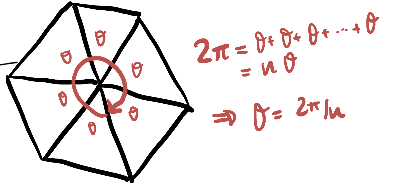
In these problems we will investigate regular polygons on the sphere. Recall we call a polygon regular if it has rotational symmetries about its center: in particular this implies that all its sides are the same length, and all its angles have the same measure (since isometries preserve both lengths and angles).
In the Euclidean plane, we know that regular polygons of all side numbers \(\geq 3\) exist (these are how Archimedes approximated the circle, after all!), but their angles are strictly determined by their number of sides. We proved in a previous homework that the angle sum of an \(n\)-gon is \((n-2)\pi\), and if all the angles of a regular \(n\) gon are equal, each angle must measure \(\theta_n = \frac{n-2}{n}\pi\).
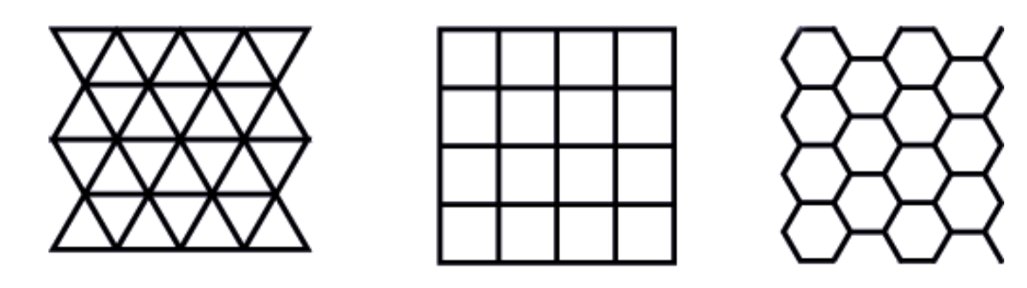
This puts a strong restriction on which regular polygons can be used to tile the plane. To tile the plane, a necessary (but not sufficient) condition is that we need to be able to fit \(k\) copies of each polygon around a vertex, without any gaps or overlaps. This tells us that the angles of a polygon that can tile must be \(\theta =\tfrac{2\pi}{k}\).
Thus, to figure out which polygons even have a chance of tiling the Euclidean plane, we want to know for which \(n\) (the number of sides) there the angle \(\theta_n\) is actually \(2\pi\) over an integer. We can start listing:
\[\theta_3=\frac{3-2}{3}{\pi}=\frac{\pi}{3}=\frac{2\pi}{6}\] \[\theta_4 = \frac{4-2}{4}\pi=\frac{\pi}{2}=\frac{2\pi}{4}\] \[\theta_5=\frac{5-2}{5}\pi=\frac{3\pi}{5}\] \[\theta_6=\frac{6-2}{6}{\pi}=\frac{2\pi}{3}\] \[\theta_7=\frac{7-2}{7}{\pi}=\frac{5\pi}{7}\]
Thus, we see that its possible to fit six triangles around a vertex, four squares around a vertex and three hexagons around a vertex, but as the angles \(\theta_5\) and \(\theta_7\) aren’t even divisions of \(2\pi\), there’s no nice way to fit pentagons or 7-gons around a vertex, and thus no hope of using them to tile the plane.
This is the start to the classification of regular tilings of the plane, where by what we see from the angle measures, its possible for triangles, squares and hexagons, but impossible for all other shapes!
Our goal here is to investigate what changes on the sphere.
Exercise 52 (Spherical Pentagons)
Find a relationship between the area \(A\) of a spherical regular pentagon and its angle measure \(\alpha\). Hint: divide the spherical pentagon into five triangles
Show that there exists a spherical pentagon whose angle evenly divides \(2\pi\): how many of these spherical pentagons fit around a single vertex?
What is the area of such a spherical pentagon? How many of these pentagons does it take to cover the entire sphere?
For the pentagon, there was only one possibility, as the restriction that the angle at a vertex be \(2\pi/k\) is so restrictive. However, for triangles, there are three possibilities!
Exercise 53 (Spherical Triangles) There are three different equilateral triangles that can be used to tile the sphere. Find them! For each triangle:
- How many fit around each vertex?
- How many are needed to cover the sphere?
- What platonic solid does this correspond to?
The Pythagorean Theorem
The fundamental formula in Euclidean trigonometry is the Pythagorean theorem which allows us to measure the length of the hypotenuse of a right triangle in terms of the other side lengths.
The goal of this exercise is to derive the spherical counterpart to this:
Theorem 2 (Spherical Pythagorean Theorem) Given a right triangle on \(\SS^2\) with side lengths \(a,b\) and hypotenuse \(c\), these three lengths satisfy the equation \[\cos(c)=\cos(a)\cos(b)\]
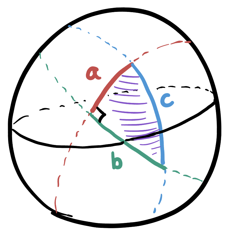
Exercise 54 (Deriving The Pythagorean Theorem) Prove that the formula given above really does hold for the legs and hypotenuse of a right triangle on \(\SS^2\), using the distance formula that we’ve already calculated:
\[\cos\dist(p,q)=p\cdot q\]
Hint: move your triangle so the right angle is at the north pole, and the legs are along the great circles on the \(xz\) and \(yz\) plane. Now you can write down exactly what the other two vertices are since you know they are distance \(a\) and \(b\) along these geodesics from \(N\), and these geodesics are unit circles in the \(xz\) and \(yz\) planes!*
On a sphere of radius \(R\), a similar formula exists: here to be able to use arguments involving angles we need to divide all the distances by the sphere’s radius, but afterwards an argument analogous to the above exercise yields
\[\cos\left(\frac cR\right)=\cos\left(\frac aR\right)\cos\left(\frac bR\right)\]
Its often more useful to rewrite this result in terms of the curvature \(\kappa=1/R^2\)
Theorem 3 (Pythagorean Theroem of Curvature \(\kappa\)) On the sphere of curvature \(\kappa\), the two legs \(a,b\) and the hypotenuse \(c\) of a right triangle satisfy \[\cos\left(c\sqrt{\kappa}\right)=\cos\left(a\sqrt{\kappa}\right)\cos\left(b\sqrt{\kappa}\right)\]
As a sphere gets larger and larger in radius, it better approximates the Euclidean plane. We might even want to say something like in the limit \(R\to\infty\) (so, \(\kappa\to 0\)) the spherical geometry becomes euclidean. But how could we make such a statement precise? One way is to study what happens to the theorems of spherical geometry as \(\kappa\to 0\); and show that they become their Euclidean counterparts. The exercise below is our first encounter with this big idea:
Exercise 55 (Euclidean Geometry as the Limit of Shrinking Curvature) Consider a triangle with side lengths \(a,b,c\) in spherical geometry of curvature \(\kappa\). As \(\kappa\to 0\), the arguments of the cosines in the Pythagorean theorem become very small numbers, so it makes sense to approximate approximate these with the first terms of their Taylor series.
Compute the Taylor series of both sides of \[\cos\left(c\sqrt{\kappa}\right)=\cos\left(a\sqrt{\kappa}\right)\cos\left(b\sqrt{\kappa}\right)\]
in the limit \(\kappa\to 0\), we can ignore all but the first nontrivial terms. Show here that only keeping up to the quadratic terms on each side recovers the Euclidean Pythagorean theorem, \(c^2=a^2+b^2\).
Trigonometry
Following the derivation of the spherical pythagorean theorem, we might next hope to discover relationships between the sides of a spherical right triangle and its angle measures. And, indeed we can!
The corresponding laws of spherical trigonometry are as follows:
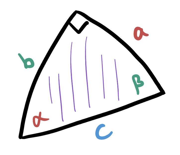
Theorem 4 (Spherical Trigonometric Relations) For a right triangle with angles \(\alpha,\beta\), corresponding opposite sides \(a,b\) and hypotenuse \(c\) the following relations hold:
\[\sin \alpha = \frac{\sin a}{\sin c}\hspace{1cm}\sin\beta =\frac{\sin b}{\sin c}\]
\[\cos\alpha = \frac{\tan b}{\tan c}\hspace{1cm}\cos\beta=\frac{\tan a}{\tan c}\]
You will not be responsible for the derivation of these formulas, nor for remembering them: if you ever need them they will be given to you!
One of the most biggest differences between spherical trigonometry and its Euclidean counterpart is that its possible to derive formulas for the length of a triangles’ sides in terms of only the angle information! This is impossible in Euclidean space because of the existence of similarities: there are plenty of pairs of triangles that have all the same angles but wildly different side lengths! No so in the geometry of the sphere.
Exercise 56 Using the trigonometric identities in Theorem Spherical Trigonometric Relations together with the spherical pythagorean theorem Theorem Spherical Pythagorean Theorem, show that the side length \(a\) of a right triangle can be computed knowing only the opposite angle \(\alpha\) and the adjacent angle \(\beta\) as
\[\cos a = \frac{\cos\alpha}{\sin\beta}\]
Hint: start with the formula for \(\cos\alpha\). Write out the tangents in terms of sines and cosines, then apply the pythagorean theorem to expand a term. Finally, use the definition of \(\sin\beta\) to regroup some terms.
Formulas such as this are incredibly useful for calculating the side lengths of polygons, by dividing them into triangles and using facts that are known about their angles.
Exercise 57 (Spherical Trigonometry) Use spherical trigonometry to figure out the side lengths of the pentagon you discovered in the first exercise.
Hint: can you further divide the five triangles you used before, into ten right triangles inside the pentagon?
Problem Set XI
Orthographic Map
Exercise 58 Can you find the coordinates \((x,y)\) of a point on the map where the vectors \(\langle 1,0\rangle\) and \(\langle 0,1\rangle\) only make a \(45\)-degree angle with one another?
Hint: can you make the problem easier for yourself by restricting \(x\) and \(y\) to lie on some line, so the problem ends up having one variable instead of two?
You can see how this would make such a map difficult to use for navigation: it would look like the map is telling you to turn \(90\) degrees but in reality you should only turn half that!
Because having to do computations like these constantly when working with a map is a huge technical headache, mathematicians much prefer conformal maps, where the angle you see in the Euclidean plane accurately represents the map-angle, and all of this is unnecessary. (This is why the main map employed by mathematicians, Stereographic Projection, is conformal).
Archimedes Map
Read the section of the textbook on Archimedes Map (in the Examples chapter). Give a proof that this mao is infinitesimal area preserving following the outline below:
Exercise 59
- Show that at each point \(p\in M\) the vectors \(\langle 1,0\rangle\) and \(\langle 0,1\rangle\) are sent by \(\psi\) to orthogonal vectors on the sphere.
- Find their lengths on the sphere (ie the map-lengths), and use this data to find the area of the infinitesimal rectangle they form.
- Observe that everything beautifully cancels and the area is still one, even though the square was stretched into a rectangle!
Since the infinitesimal area is unchanged by the map at each point, we can finish Archimedes proof via integration (which I do below, using your exercise)
Theorem 5 The surface area of the unit sphere is the same as that of its Archimedes map: that is, the same as the area of its bounding cylinder.
Proof. Archimedes map captures every point of the sphere except the north and south poles. Since points have zero area, this omission has no effect on our actual question so we can proceed to calculate with the map \(M\).
\[\area(\SS^2)=\iint_{\SS^2} dA_{\SS^2}=\iint_{\psi(M)}dA_{\SS^2}= \iint_{M}dA_{\map}\]
But now we know that \(dA_{\map}=dA_{\EE^2}\), that’s what you’ve proved in the exercise above! So we can sub this out, and then realize the resulting integral is just the definition of the Euclidean area of \(M\) in the plane:
\[=\iint_M dA_{\EE^2}=\area(M)\]
Stereographic Projection:
Read the stereographic projection section first (we will cover the necessary bits in class as well)
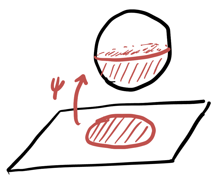
The stereographic projection map has many uses in mathematics beyond just representing points of the sphere on the plane. Because it is conformal (angle preserving), its often used as a tool to help build more interesting conformal maps between regions of the plane, following this general recipe:
- Start with a region on the plane.
- Use \(\psi\) to map it to the sphere.
- Do something to the sphere, moving the region around
- Use \(\phi\) to put it back on the plane.
The overall composition is a map between two regions on the plane, that was created by going to the sphere and back! In these exercises, we will deal with a fundamental example of this, and construct a map from the unit disk onto half of the entire plane!
The strategy above is summarized for this case in the following three figures:
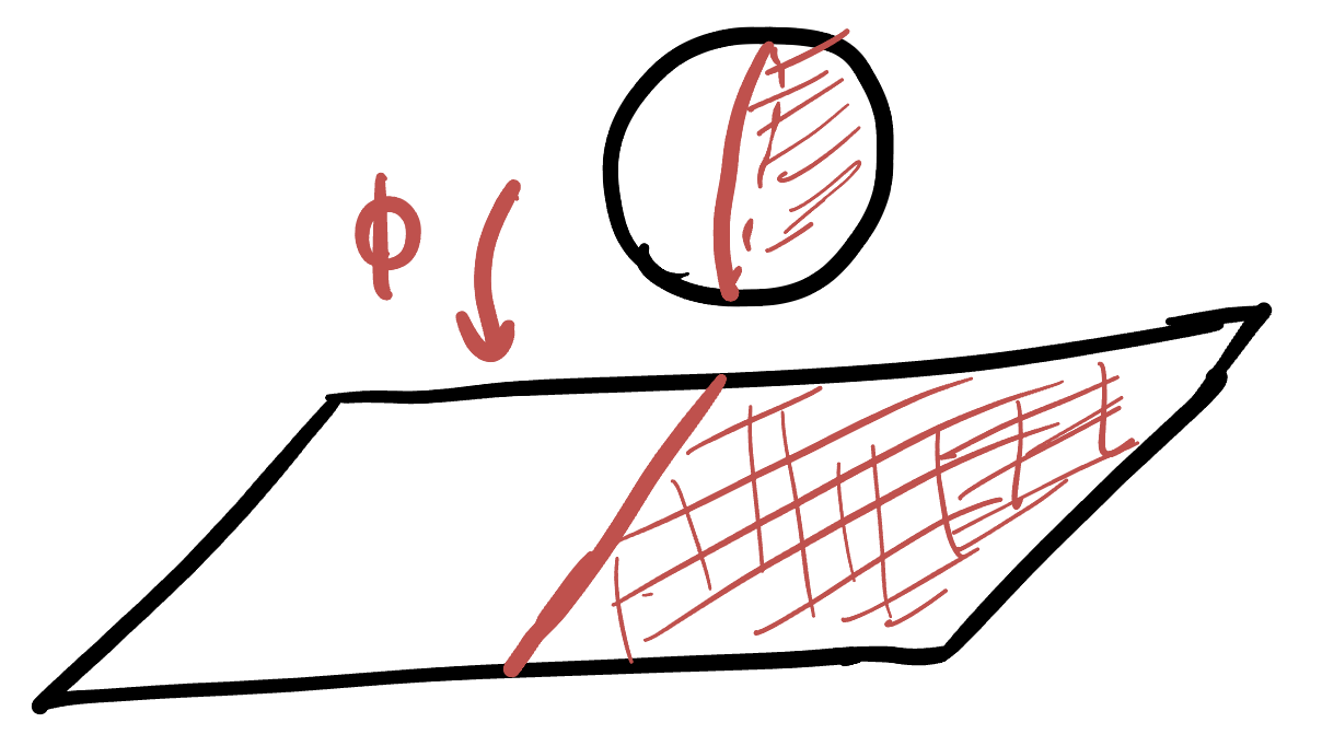
Exercise 60 (Disk and Half Plane: Construction) Let \(\DD\) be the unit disk \(\DD=\{(x,y)\mid x^2+y^2<1\}\) and let \(\mathbb{U}\) be the upper half plane \(\mathbb{U}=\{(x,y)\mid y>0\}\). Let \(T\colon \DD\to \mathbb{U}\) be the map described above. Prove that $T can be expressed as
\[T(x,y)=\left(\frac{2x}{1+x^2+y^2-2y},\frac{1-x^2-y^2}{1+x^2+y^2-2y}\right)\]
By building it step by step:
- Start with \((x,y)\) in the unit disk.
- Apply \(\psi\) to get the disk onto the sphere.
- Rotate the sphere about the \(x\) axis in the appropriate way so that the south pole goes to \((0,1,0)\).
- Apply \(\phi\) to return to the plane.
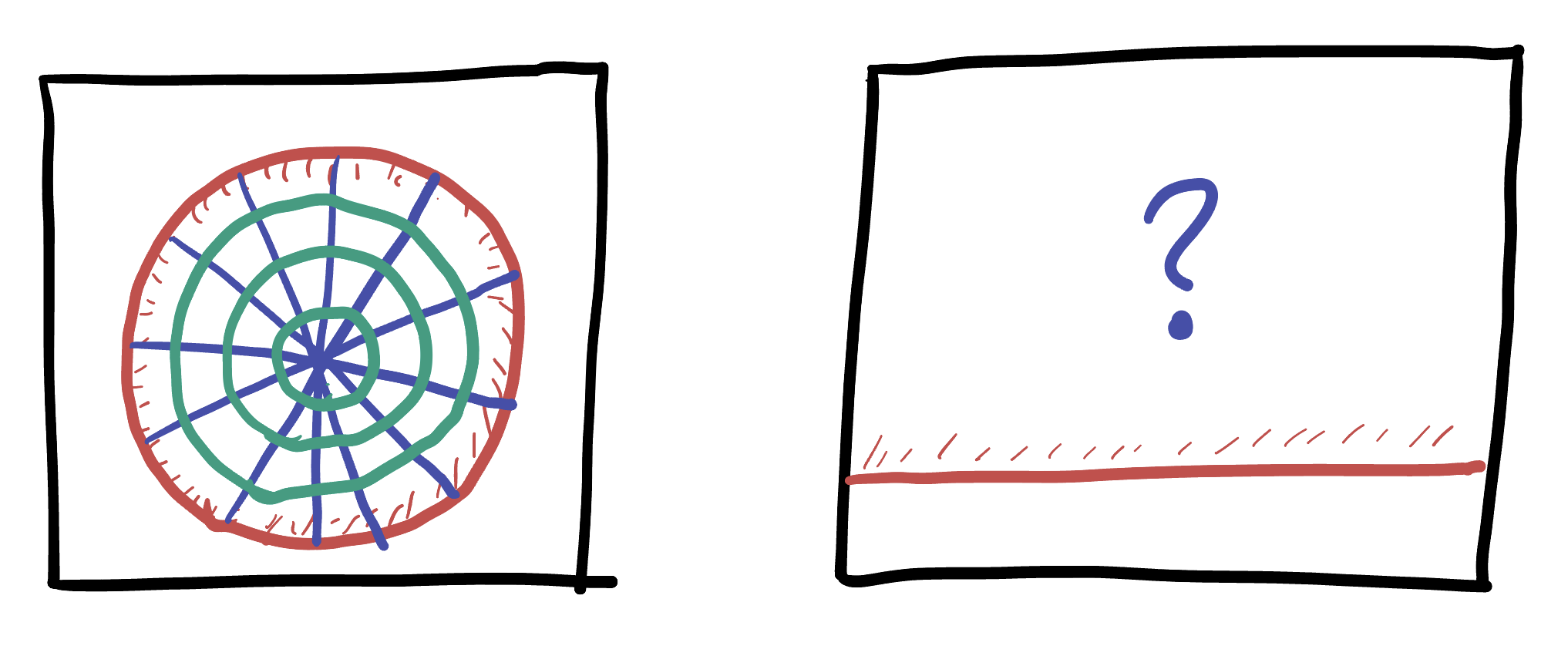
This map is conformal - meaning that it preserves all angles! And even more than that, it takes generalized circles to generalized circles.
Exercise 61 (Disk and Half Plane: Understanding) Prove that these claims are in fact true: that our new function is conformal, and sends generalized circles to generalized circles. Hint: what kinds of maps is it built out of? What do each of these maps to do angles, or to generalized circles (on the plane) / circles (on the sphere)?
Use this to “transfer” this picture of polar coordinates in the unit disk onto the plane, via our new map.
Spheres of Radius \(R\):
The chapter on stereographic projection deals with the unit sphere. It is not too hard to generalize what we have done to spheres of other radii, and while this may not sound super exciting at first, it actually turns out to be absolutely fundamental to how we are going to discover hyperbolic space! So, it is a rather important exercise to work this all out for yourself.
The good news is you have this entire chapter as a guide, where I’ve worked out many of the details for the case of the unit sphere. The formulas will be quite similar, but there’ll be \(R\)’s inserted in various places: so the second piece of good news is that I’ll give you the formulas that you need to derive! That way, you can check your work.
Definition 6 Let \(\SS^2_R\) be the sphere of radius \(R\) in \(\EE^3\). Then the chart \(\phi\) for stereographic projection of this sphere is defined geometrically exactly as in the original version: given a point \(p\in\SS^2_R\), \(\phi(p)\) is where the line connecting \(p\) to the north pole \(N=(0,0,R)\) intersects the \(xy\) plane.
Exercise 62 Show that the formulas for both the chart and the parameterization of stereographic projection here are as follows:
\[\phi(x,y,z)=(X,Y)=\left(\frac{Rx}{R-z},\frac{Ry}{R-z}\right)\]
\[\psi(X,Y)=(x,y,z)=\left(\frac{2R^2 X}{X^2+Y^2+R^2},\frac{2R^2 Y}{X^2+Y^2+R^2},R\frac{X^2+Y^2-R^2}{X^2+Y^2+R^2}\right)\]
(It might help to look back at Proposition Stereographic Projection Formula, and attempt Exercise exr-stereo-parameterization).
Running through the same arguments as in the chapter above (which you don’t have to write down), its straightforward to check that this new map is a conformal map between \(\SS^2_R\) minus \(N\), and the plane. This means its parameterization \(\psi\) both preserves angles and stretches all vectors by a uniform length: we can use this fact to compute the dot product for this map.
Exercise 63 At a point \(p=(X,Y)\) on the plane, what is the factor by which a vector \(v\in T_p\EE^2\) is stretched when mapped onto \(\SS^2_R\) by the parameterization of stereographic projection? Hint: we know the factor is the same for all vectors: so pick an easy vector to calculate with and find its length!
Once you know this, follow the argument style of Theorem Stereographic Dot Product to compute the map-dot product on the plane, and show that it is equal to
\[(v\cdot w)_\map = \frac{4R^4}{(R^2+X^2+Y^2)^2}(v\cdot w)\]
Problem Set XII
Getting Used to Hyperbolic Space
Exercise 64 (Hyperbolic Circle Area) In this exercise you will go through the transition-style arguments we use to turn formulas on the sphere into their analogs in hyperbolic geometry, much like we did in class.
The starting point is the formula for the area of a circle of radius \(r\) on the sphere of radius \(R\):
\[A(r)=\int_0^r C(r)dr=\int_0^r 2\pi\sin\left(\frac{r}{R}\right)dr=2\pi R^2\left(1-\cos\frac{r}{R}\right)\]
- Re-express this in terms of curvature
- Convert to the Taylor series
- Plug in \(\kappa=-1\)
- Convert back to hyperbolic trigonometric functions
What is the correct hyperbolic formula? (We wrote it down without doing the full derivation in class, so you can confirm)
Exercise 65 (Hyperbolic Pizza) One way to try and develop intuition for the strange behavior of circles is to think about the type of circles we see in daily life: pizzas! One major factor determining how good a pizza is is its crust percentage which we will define as \[\mathrm{CrustPercent}=\frac{\area(\mathrm{Crust})}{\area(\mathrm{Pizza})}\]
In this probelm we will consider pizzas which have 1 inch crusts: meaning a 10 inch (radius) pizza has a 9inch radius center of toppings, surrounded by a 1 inch thick circle of crust.
- Show the CrustPercent for Euclidean pizza is \[\frac{2}{r}-\frac{1}{r^2}.\] From this we see that as \(r\to \infty\) the crust percent drops to zero: this makes sense, if you imagine an extremely large pizza with only a 1inch thick crust, it’s totally reasonable that most of the pizza is not crust!
- What is the CrustPercent for a hyperbolic pizza of radius \(r\)? Show that when \(r\) is large, this limits to the constant \[\mathrm{CrustPercent}\to 1-\frac{1}{e}\approx 63\%\] Thus crust is an inevitable part of life in hyperbolic space: no matter what size pizza you make it will always be well over half crust!
Exercise 66 (Hyperbolic Pizza II) In this problem, we will imagine our unit to be inches (so, the radius appearing in formulas for space of curvature \(-1\) is measured in inches).
You are at a pizzerias and are trying to decide if the 5 inch radius pizza they sell is large enough for you and your friends. They also sell a six inch (radius) pizza, but it costs twice as much. At first, you think this sounds crazy! But is this actually a good deal, or not?
Your friend is feeling very hungry, and jokingly asks the pizza-maker how large of a pizza he would need to order so that its areas is the same as an american football field (\(100\times 50\) yards). The pizza-maker says “I think I have room for that in my oven, coming right up!” How big of a pizza is he going to make?
Hint: invert the formula for area in terms of radius, to get radius in terms of area, then plug into a calculator!
Working with the Models
Exercise 67 (Hyperbolic space is homogeneous) We proved in class that the horizontal translations \(T(x,y)=(x+t,y)\) are isometries of the Half Plane model, and we also proved that the similarities \(S(x,y)=(sx,sy)\) are also isometries.
Combining these two, prove that \(\HH^2\) is homogeneous: that is, that for any two points \(p,q\in\HH^2\), there exists an isometry that takes \(p\) to \(q\).
Hint: can you first show that you can build an isometry that takes \((0,1)\) to any point in the plane? Then combine two of these to get what you want?
Exercise 68 (The Circumference of Circles) In the Disk Model, if \(a<1\) the Euclidean circle \(x^2+y^2=a^2\) centered at \(O\) is also a hyperbolic circle. In the text, we compute that its hyperbolic circumference is
\[C = \frac{4\pi a}{1-a^2}\] and that its hyperbolic radius is
\[r=2\mathrm{arctanh}(a)\]
Using these two, prove that \(C(r)=2\pi\sinh(r)\). Hint: solve for \(a\) in terms of \(r\) and plug into circumference. Then use hyperbolic trigonometric identities to simplify!
Together these two arguments prove that the geometry modeled by the Half Plane and the Disk has the circumference function \(C(r)=2\pi\sinh(r)\) for circles based at any point (the second problem establishes this for circles at a special point, and hte first problem establishes that space is homogeneous, so its the same at all points). Thus, this space truly is hyperbolic geometry, and has curvature \(-1\) (we proved in class, any space with this circumference function has constant curvature \(-1\)).